BigQuery - Quick Guide

---

---

BigQuery - Overview

BigQuery is Google Cloud Platform's (GCP) structured query language (SQL) engine. BigQuery allows users to query, create and manipulate datasets instantly using serverless cloud infrastructure. Consequently, students, professionals and organizations gain the ability to store and analyze data at a nearly infinite scale.

Like several other Google initiatives, BigQuery began as an in-house tool for Google developers to process and analyze large datasets. Googlers have been using BigQuery and its predecessor, Dremel, since 2006. Finding success within Google, GCP first released BigQuery as a beta in the year 2010 and then made the tool widely available in 2011.

How did BigQuery Edge Over Its Competitors?

Although there were many SQL engines and integrated development environments (IDEs) in the market at the time of BigQuery's release, BigQuery leveraged several competitive advantages, among them −

• Pioneering a slot-based query system, which could automatically allocate compute power or "slots" based on user demand
• Offering API integrations with a variety of programming languages from Python to JavaScript
• Providing users the ability to train, run and deploy machine learning models written in SQL
• Integrating seamlessly with visualization platforms like Google Data Studio (deprecated) and Looker
• The ability to store and query ARRAY and STRUCT types, both complex SQL data types

To assist students and professionals, BigQuery maintains robust documentation about functions, public datasets and available integrations.

Google BigQuery Use Cases

Wielded properly, Google BigQuery can be used as a personal or organizational data warehouse. However, since BigQuery is SQL-oriented, it is best used with sources that feature structured, not unstructured, data.

Google's cloud architecture facilitates reliable storage and enables nearly infinite scalability. This makes BigQuery a popular enterprise choice, especially for organizations that generate or ingest large volumes of data.

To truly understand the power of BigQuery, it is helpful to understand how use cases differ between the various data team roles.

• Data Analyst − Employs BigQuery in conjunction with data visualization tools like Tableau or Looker to create top-line reports for organizational leadership.
• Data Scientist − Leverages BigQuery's machine learning capabilities, Big ML, to create and implement ML models.
• Data Engineer − Uses BigQuery as a data warehouse and builds tools like views and user defined functions to empower end users to discover insights in cleaned, preprocessed datasets.

When used in tandem, BigQuery presents an opportunity to optimize storage and generate nuanced insights to increase growth and revenue.

Loading Data in BigQuery

Loading data in BigQuery is simple and intuitive with a variety of options available to cloud developers. BigQuery can ingest data in many forms including −

• CSV
• JSON
• Parquet

BigQuery can also sync with Google integrations like Google Sheets to create live connected tables. And BigQuery can load files stored in cloud storage repositories like Google Cloud Storage.

Developers can also leverage the following methods to cleanly load data into BigQuery −

• BigQuery Transfers, a code-less data pipeline that integrates with GCP data like Google Analytics.
• SQL-based pipelines that feature CRUD statements to CREATE, DELETE or DROP tables.
• Pipelines that utilize the BigQuery API to conduct batch or streaming load jobs.
• Third-party pipelines like Fivetran that offer BigQuery connections.

Routinely loading data from the above sources enables downstream stakeholders to have reliable access to timely, accurate data.

BigQuery Querying Basics

While it is helpful to understand BigQuery use-cases and how to properly load data, beginners learning BigQuery will most likely start at the query layer.

Table Reference Convention in BigQuery

Before writing your first SELECT statement, it is helpful to understand table reference convention in BigQuery.

BigQuery syntax differs from other SQL dialects because proper BigQuery SQL requires developers to enclose table references in single quotes like this − ' '.

A table reference involves three elements −

• Project
• Dataset
• Table

Put together, a BigQuery table looks like this when referenced in a SQL query or script −

'my_project.dataset.table'

A basic BigQuery query looks like this −

SELECT * FROM 'my_project.dataset.table.'

Legacy SQL and Standard SQL

An important distinction between BigQuery SQL and other types of SQL is that BigQuery offers support for two classifications of SQL: Legacy and Standard.

• Legacy SQL enables users to use older, possibly deprecated SQL functions.
• Standard SQL represents a more updated interpretation of SQL.

For our purposes, we'll be using the standard SQL designation.

Points to Note When Writing a Query in BigQuery

Unlike other SQL environments, when you write a query in BigQuery, the UI will automatically tell you whether your query will run and how much data it will process. Note that there is little definitive correlation between volume of data processed and projected execution time.

• Once executed, your query will return a result visible in the UI, which is similar to viewing a spreadsheet or a Pandas data frame.
• You also have the option to download your result as either a CSV or JSON file, which both provide a simple way to save data to work with later.
• If you need to save query text to run or edit later, BigQuery also provides an option to save queries with version control to help track changes.

Running BigQuery at the Enterprise Level

When running queries in an organization with several BigQuery users, it is important to keep in mind several factors to ensure your queries run without interruption or without causing congestion for other users −

• Avoid executing queries at peak usage times.
• Whenever possible, use a WHERE clause to narrow the amount of data processed.
• For large tables, create views users can more easily and efficiently query.

Transitioning from learning BigQuery to running queries at the enterprise level requires time to develop an understanding of variables particular to your organization like slot usage and compute resource consumption.

First, however, it is necessary to develop a deeper understanding of constructing and optimizing queries in BigQuery.

BigQuery - Initial Setup

To try some of the following concepts, it is necessary to create a Google Cloud Platform account. By creating a GCP account you will gain access to Google's suite of cloud applications, including BigQuery.

In order to expose GCP products to a wide audience, Google has added free usage tiers for many of its flagship products, including BigQuery. BigQuery users, regardless of the pricing plan, can query up to 1 terabyte (TB) of data and store up to 10 gigabytes (GB) free per month.

However, to avoid having to attach a credit card to your account and incurring even incidental charges, it's possible for new users to enroll in a 90-day free trial period. The free trial comes with $300 worth of GCP credit. Truthfully, unless users are running computationally-heavy processes like virtual machines or deploying ML models, this is more than enough.

According to Google, a user is eligible for the program provided they −

• Have never been a paying customer of Google Cloud or affiliated products
• Have not previously signed up for a Google Cloud Platform free trial

To sign up for a 90-day trial of BigQuery, take these steps: Navigate to cloud.google.com/free You should see this page.

Click "Get started for free" (center of page)

Sign into your Google account −

Once you complete the signup flow, you'll gain access to Google Cloud Platform.

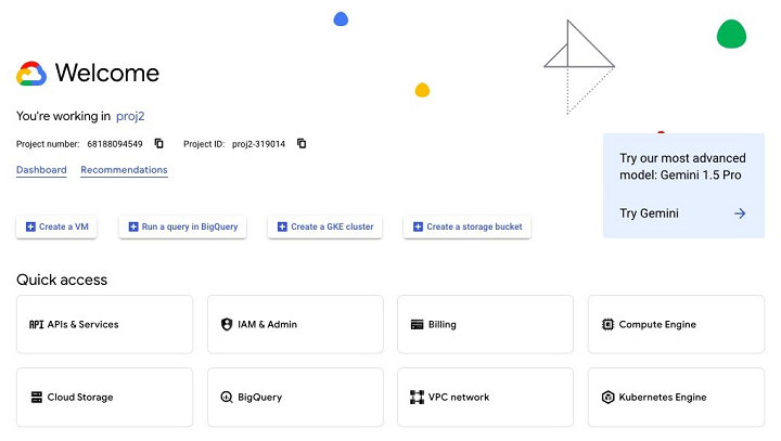
The first thing you'll see each time you log in is the GCP logo with "Welcome." At the bottom of the "welcome" page, you'll see "Quick Access" links to your frequently used GCP applications.

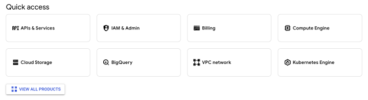
Additionally, you'll be able to access all the features of BigQuery that this tutorial will highlight and explore.

BigQuery vs Local SQL Engines

With SQL being around for 40+ years, BigQuery was not the first SQL environment. Prior to BigQuery's release, SQL developers worked primarily with on-premises or "on-prem" databases.

The systems that allow developers to manage and interact with databases are called database management systems (DBMS).

In the days before the "cloud engineer" or "data engineer" job title gained popularity and widespread use, those who worked with DBMS tools held titles like "architect." Often, this title was used quite literally, as those who worked with databases maintained both physical and digital infrastructure.

Data Modeling

As database technology evolved, an architect's responsibilities primarily concerned a task called data modeling.

While functions like INSERT() can make it seem easy to take data from a source and add it to a database, in organizations that embrace data modeling, there is a lot of thought involved in how to store and mold the data.

Popular data modeling concepts include phrases like "star schema" or "normalization" and "normal forms."

How is BigQuery Different from any Traditional DBMS?

While it is still advised to follow best practices when creating BigQuery tables, BigQuery is a bit more out-of-the-box than traditional DBMS interfaces.

BigQuery differs from a more "traditional" DBMS in the following ways −

• Scalability − BigQuery can scale to meet nearly any storage or querying need, thanks to the staggering amount of cloud storage made available by Google's data centers.
• API integration − BigQuery's SQL engine can be leveraged programmatically, while DBMS like Postgre can only run native SQL queries.
• ML/AI capabilities, integrating with Vertex AI.
• More specific data types available for long-term storage.
• A Google-specific SQL dialect, Google Query Language (GQL) that includes more specialized functions than more legacy SQL dialects.

From a user's perspective, BigQuery also offers more visibility regarding execution stats and user activity −

• Allowing users to see if a query is acceptable before executing accompanying SQL
• Providing execution plans and query lineage
• Expanded metadata stores to provide insight into query usage, storage and cost

BigQuery truly is the standard for cloud-based SQL querying, which begins in The Google Cloud Console.

BigQuery - Google Cloud Console

Since BigQuery is a cloud-based data warehouse and querying tool it can be accessed anywhere through the Google Cloud Console. Unlike a localized database like, say, PostgreSQL or MySQL, Google did not create an app for BigQuery. Instead, BigQuery lives "in the cloud" within the Google Cloud Console.

Google Cloud Console: Homepage for All GCP Applications

If you've created a Google account and associated GCP project, you'll gain access to the Google Cloud Console.

To navigate to BigQuery, you can either type "BigQuery" in the search bar or select it from the pop-out menu on the left of the Google Cloud Console, where you'll find it under the "Analytics" category.

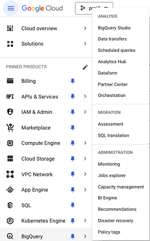
To ensure access throughout this tutorial, it is recommended that you pin it to designate "BigQuery" as a pinned product within your environment.

Through the console, you'll be able to access all aspects of BigQuery, including −

• BigQuery Studio
• The BigQuery API
• Logs & errors pertaining to BigQuery
• Billing for BigQuery slot usage

Just as you would set up an IDE to meet your standards of comfort and efficiency, it is highly recommended you take the time to customize your Google Cloud Console experience to be able to quickly and reliably access relevant BigQuery resources.

BigQuery - Google Cloud Hierarchy

Before proceeding, it's important to grasp the fundamental concepts and vocabulary relating to BigQuery and its associated processes.

First, it's important to understand that even though cloud computing offers nearly limitless processing capabilities, BigQuery users will encounter issues if they are required to do the following activities −

• Performing a computationally-taxing SQL operation like a cross join or cartesian join.
• Attempting to run a large query without specifying a destination table.
• Running a large query at times of peak usage (if using BigQuery as an enterprise user).
• On-demand or "ad hoc" queries can and will create gridlock, especially if competing with scheduled processes for execution slots.

Google Cloud Hierarchy

If you anticipate creating and populating data sources within BigQuery, it is important to note the Google Cloud hierarchy −

• Organization
• Project
• Dataset
• Table

1. Organization Layer

Unless you are an account owner, executive or decision maker, you're unlikely to have to worry about the organization layer. Think of it as the entity that contains the other elements you'll encounter when navigating BigQuery Studio and writing SQL queries within the SQL environment.

2. Multiple Projects Inside Google Cloud Organization

Any Google Cloud organization can have multiple projects. Sometimes companies or enterprise users (we'll purposefully avoid the term "organization" here to avoid confusion) create different projects to separate staging and production environments.

Other times, these high-level users create distinct projects to have more control over potentially sensitive data like personally identifiable information (PII) and confidential revenue information.

In either case, when you begin using BigQuery, you'll create or receive permissions to access BigQuery as a user with specific permissions and role scopes.

3. Datasets and Tables within Project

Within the project, the most important entities to remember are datasets and tables. To clarify, a dataset contains a table or multiple tables. In order to maintain accuracy in technical discussions, do your best to avoid using these terms interchangeably.

Other elements you'll see within a dataset include −

• Routines
• Models
• Views

These additional data elements will be discussed in more depth in the following chapters.

What is Dremel?

BigQuery is not a limitless tool. In fact, it is better to avoid thinking of BigQuery as a proverbial black box. To deepen your understanding, it's necessary to get a bit "under the hood" and examine some inner workings of BigQuery's engine.

Google's Dremel: A Distributed Computing Framework

BigQuery is based on a distributed computing framework called Dremel, which Google explained in greater depth in a 2010 whitepaper: "Dremel: Interactive Analysis of Web Scale Datasets."

The whitepaper described a vision for many of the core characteristics that define modern BigQuery such as an ad-hoc query system, nearly limitless compute power, and an emphasis on processing big data (terabytes & petabytes).

How does Dremel Work?

Since Dremel was first an internal product (used within Google since 2006), it combines aspects of search and a parallel database management system.

To execute queries, Dremel used a "tree-like" structure in which each stage of the query is executed in sequential steps and multiple queries can be executed in parallel. Dremel turns the SQL queries into an execution tree.

Slots: Foundational Unit of BigQuery Executioin

Nestled under the "Query Execution" header, the authors describe the foundational unit of BigQuery execution: the slot.

• A slot is an abstraction that represents an available processing unit.
• Slots are finite, which is why any logjams within a project are often due to a lack of slot availability.
• Since the usage of slots changes depending on many factors like the volume of data processed and time of day, it's conceivable that a query that executed quickly earlier in the day may now take several minutes.

The abstraction of slots is perhaps the most applicable concept expressed in the Dremel paper; the other information is helpful to know but mostly describes earlier iterations of the BigQuery product.

BigQuery: Pricing & Usage Models

Whether you're a student practicing your first BigQuery queries or a high-powered decision maker, understanding pricing is critical in defining the limits of what you can store, access and manipulate within BigQuery.

To thoroughly understand BigQuery pricing, it is best to divide the costs into two buckets −

• Usage (BigQuery's documentation calls this "compute")
• Storage

Usage covers nearly any SQL-activity you can think of, from running a simple SELECT query to deploying ML models or writing complex user-defined functions.

For any usage-related activities, BigQuery offers the following choices −

• A pay as you go or "on-demand" model.
• A bulk slot or "capacity" model in which clients pay per slot hour.

Which Pricing Model is best for you?

When it comes to deciding between the two pricing models, it is important to consider the following factors −

• Volume of data queried
• Volume of user traffic incurred

The "on-demand" model is priced per terabyte, which means that for users with many large (multiple terabyte) tables this could be an intuitive and convenient way to track expenses.

The "capacity" or slot model is helpful for organizations or individuals that are evolving their data infrastructure and may not have a fixed amount of data that would help them calculate a reliable per-month rate. Instead of worrying about how much data each resource generates, the problem shifts to refining best practices to allocate querying time to both scheduled processes and individual, ad-hoc queries.

In essence, the slot model follows the framework established by the Dremel project, in which slots (servers) are reserved and priced accordingly.

What is BigQuery Studio?

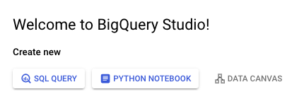
Having established a baseline product knowledge and theory, it's time to return to the Google Cloud Console and enter BigQuery Studio. Once simply called "SQL workspace", BigQuery Studio is where users will run not just BigQuery queries, but also a range of other data and AI workflows.

BigQuery's goal is to provide a space that mirrors GitHub in that it provides users the ability to write and deploy SQL, Spark and even Python code while maintaining version history and facilitating collaboration among data teams.

SQL Query, Python Notebook, Data Canvas

Opening BigQuery Studio for the first time is reminiscent of any other SQL IDE. However, unlike a local SQL IDE, you're given three choices for actions when BigQuery opens −

• SQL Query
• Python Notebook
• Data Canvas

Clicking SQL query should open a blank page on which you can write and run queries. Consequently, the SQL query and Python notebook options should be self-explanatory. Data canvas is an AI integration that won't be covered in this tutorial.

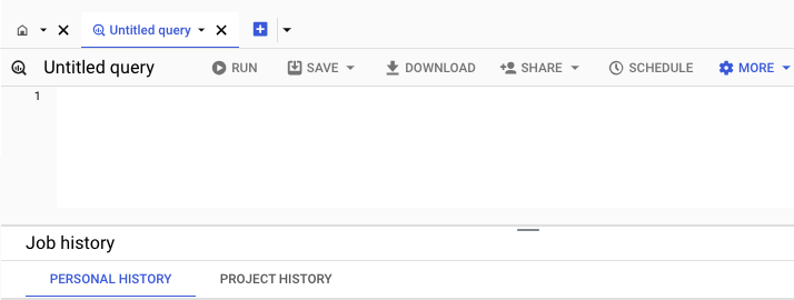
Assuming you've created or have access to a BigQuery project, on the left menu, you'll see a drop-down of the project name followed by any datasets within that project's scope.

Click into any of those datasets and you'll see the tables created within that dataset.

At the bottom you'll see information related to the SQL jobs you run. These jobs are split into "personal", or queries created and run by your profile, or "project", which allows you to see all the metadata for jobs run within the project.

Saving work within BigQuery Studio can be achieved either without version history, a "classic" saved query, or with version history. The save feature also allows for the easy creation of views, which will be covered in more depth in later chapters.

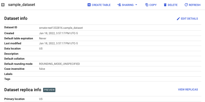
BigQuery - Datasets

Datasets are entities that live within a project. Datasets act as a container for BigQuery tables as well as views, routines and machine learning models.

Tables cannot live separately from datasets, so it is a requirement to create a dataset when creating a new data source within BigQuery Studio.

In addition to attributes like a human-readable name, developers are required to specify a location when authorizing the creation of a dataset. These locations correspond with the physical locations of Google data centers throughout the world.

When specifying a location, you'll need to specify either a single region or multi-region. For instance, instead of choosing a data center in Chicago, you would specify "us-central-1."

Establishing a dataset as a multi-regional entity provides the added advantage of BigQuery shifting the location when a particular region does not have the resources to keep up with current demand. The current multi-regions are located in either the Americas (U.S.) or EU (Europe).

Steps to Create a Dataset in BigQuery

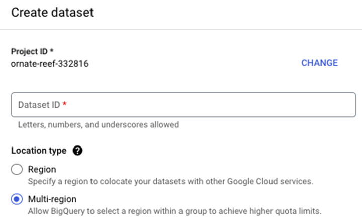
To create a dataset, follow the steps given below. First, navigate to your project name and click the three dots which will trigger a pop-up with "create dataset" −

Once you click "create dataset", you'll be prompted to enter −

• A dataset_id
• A location type (region vs. multi-region).
• A default table expiration (how many days until the table expires).

The end result is a dataset which serves as a container for future tables, views and materialized views.

A "Sharing" option allows developers to manage access control to datasets in order to limit unauthorized users.

BigQuery: Public Datasets

If you're new to BigQuery and, possibly, SQL in general, it's likely you may not have generated data to store and manipulate. This is one of the advantages of using BigQuery Studio as a SQL sandbox. In addition to serverless infrastructure, BigQuery also provides terabytes of sample data that students and professionals can use to learn and refine their SQL skills.

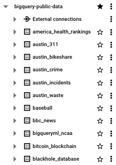
• Published through the Google Cloud Public Dataset Program, BigQuery public datasets are stored in their own universally-accessible project: bigquery-public-data.
• Developers can query up to 1 terabyte of data per month for free, in accordance with the pay-per-terabyte pricing model.
• Unlike many stock datasets, the data contained within the tables is realistic, a.k.a. "messy" and, at times, requires significant transformation to yield actionable insights.

BigQuery also provides several sample tables independent of its BigQuery public datasets which can be found in the bigquery-public-data:samples table dataset −

• gsod
• github_nested
• github_timeline
• natality
• shakespeare
• trigrams
• wikipedia

Perhaps the most significant advantage of accessing BigQuery public datasets is the fact that the data is ingested from real data sources like the BBC, Hacker News and Johns Hopkins University.

BigQuery - Tables

Tables are the foundational data source of BigQuery. BigQuery is a SQL data store, so data is stored in a structured (as opposed to unstructured or NoSQL) manner. BigQuery SQL tables are columnar, following a similar structure as a spreadsheet, with attributes or fields mapped to columns and records populating rows.

Unlike datasets, when creating a table, users do not have to specify a location.

Types of Tables in BigQuery

There are two important table types within BigQuery −

• Standard tables (like any SQL-oriented table).
• Views (a semi-permanent table that can be queried like a standard table).

Table Example

Table creation will be covered in a later chapter. In the meantime, however, it is helpful to recognize and identify the table types discussed above.

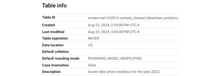
This is an example of a standard table −

Notably, users can see a metadata attribute, "Description", that immediately informs the developers and users what data the table contains.

View Example

Creating or having access to a table enables developers to build subsequent resources based on this data source. One table type you'll undoubtedly encounter and work with is a view.

This is how a view appears in BigQuery.

Its schema and appearance in the UI is nearly identical to that of a standard table.

Finally, views are created using a view definition, which is really just a materialized query.

BigQuery - Views

What are Views in SQL?

In SQL, a view is a virtualized table that, instead of containing the output of a data source like a CSV file, contains a pre-executed query that updates as new data is available.

Since views contain only pre-filtered data, they are a popular method for reducing the scope of volume processed and, by extension, can also reduce the execution time for certain data sources.

• While a table is the totality of a data source, a view represents a slice of data generated by a saved query.
• While a query might SELECT everything from a given table, a view might contain only the most recent day's data.

Creating a BigQuery View

BigQuery views can be created by a data manipulation language (DML) statement −

CREATE OR REPLACE VIEW project.dataset.view

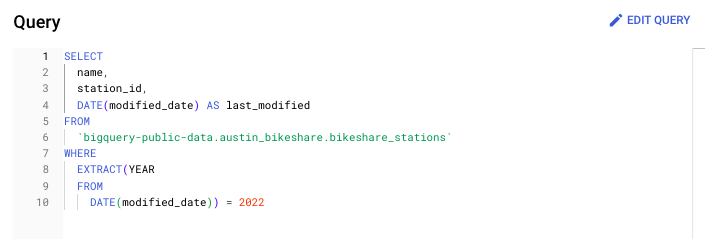
Here is an example of creating a view definition containing Austin Bikeshare station data (from the BigQuery public dataset of the same name) for only the year 2022.

Alternatively, BigQuery users can create views within the BigQuery user interface (UI). After clicking on a dataset, instead of selecting "create table", simply select "create view." BigQuery provides a separate icon to distinguish standard tables and views so developers can tell the difference at a glance.

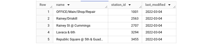
To access the view we created above, simply run a SELECT statement like you would use to access data generated within a standard table.

With this query, you will get an output table like the one shown here −

Materialized Views

In addition to standard views, BigQuery users can also create materialized views. A materialized view sits between a view and standard table.

BigQuery documentation defines materialized views as: "[P]recomputed views that periodically cache the results of the view query. The cached results are stored in BigQuery storage."

It's important to note that standard views do not indefinitely store data and, consequently, do not incur long-term storage fees.

BigQuery - Create Table

To start leveraging the power of BigQuery, it's necessary to create a table. In this chapter, we will demonstrate how you can create a table in BigQuery.

Requirements for Creating a BigQuery Table

The requirements for creating a BigQuery table are −

• Table source ("create table from")
• Project
• Dataset
• Table name
• Table type

Example: Creating a BigQuery Table

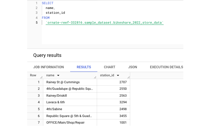
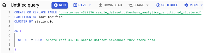
Returning to the Austin Bikeshare data set, we can run this CREATE TABLE statement.

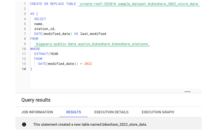
This statement created a new table called bikeshare_2022_store_data. Next, let's run a query to extract some data from this newly created table −

Additionally, tables can be partitioned and clustered, which are both storage methods that can help increase the efficiency of table storage and querying.

Finally, tables generate and contain helpful metadata to let developers know when their contents were last altered (the last modified field), offer a brief description of the table's purpose or even dictate how long until table data expires (partition expiration days).

BigQuery - Basic Schema Design

Unlike an Excel spreadsheet, SQL tables do not automatically accept data as it is presented. The data source and table must be in agreement about the data's scope and types before ingestion can be successful. Types must be both consistent and in a format that BigQuery can parse and make available within BigQuery Studio.

What is a Schema?

To do this, developers must provide a schema. Essentially, a schema is an ordered list of attributes and their corresponding types.

In BigQuery, column order and the number of columns matters, so any supplied schema must match that of the source table.

Three Ways to Specify a Schema

In BigQuery, there are three ways to specify a schema −

• Create a schema within the UI during the "create table" step.
• Write or upload a schema as a JSON text file.
• Tell BigQuery to auto-infer the schema.

Auto-infer the Schema

While auto inferring a schema is the least work for a developer, this can also introduce the most risk into a data pipeline.

Even if data types are consistent on one run, they could change unexpectedly. Without a fixed schema, BigQuery has to "figure out" which data type to accept, which can lead to schema mismatch errors.

The UI Method of Creating a Schema

Since the UI method of creating a schema is rather intuitive, the next part will focus on creating a schema as a JSON file.

Creating a Schema as a JSON File

The format for JSON schema is a dictionary "{ }" inside of a list "[ ]." Each field can have three attributes −

• Field Name
• Column Type
• Column Mode

The default column mode is "NULLABLE" which means the column accepts NULL values. Other column modes will be covered during the discussion of nested data types.

An example of one line of a JSON schema would be −

{"name": "id", "type": "STRING", "mode": "NULLABLE"}

If you're simply adding a column or altering the type of an existing column, you can generate the schema of an existing table with this query −

[Generate schema query]

Just make sure results are set to "JSON" to copy/download the resulting JSON file.

GCP Cloud Shell: Create a Table

Cloud Shell is Google Cloud Platform's command line interface (CLI) tool that allows users to interact with data sources directly from a terminal window. Just as it's possible to create a table using the BigQuery UI in the GCP Console, it is possible to quickly create a table using a Linux-like syntax via the CLI.

Unlike provisioning a CLI on a local machine, as long as you're logged into a Google account, you're automatically logged into the Cloud Shell and, consequently, can interact with BigQuery resources in the terminal. It is also possible (but more complex) to provision the gcloud CLI in a local IDE.

The "bq" Command-line

In either case, the BigQuery cloud shell integration hinges on one command: bq. The bq command-line is a Python-based command line tool compatible with cloud shell.

To create a table, it is necessary to use "bq" in combination with "mk" −

--bq mk 

This syntax is used in combination with the "table" or "-t" flag. There is also the option to specify multiple parameters, just like when creating a table within the BigQuery UI.

Available parameters include −

• Expiration rules (expiration time in seconds)
• Description
• Label
• Add tags (policy tags)
• Project id
• Dataset id
• Table name
• Schema

Here is an example −

Note − An inline schema was provided.

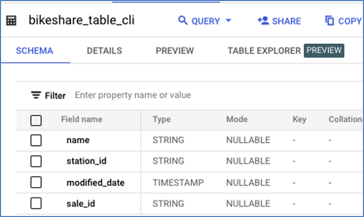
Bq mk -t sample_dataset.bikeshare_table_cli
name:STRING,station_id:STRING,modified_date:TIMESTAMP

After successful execution, you will get an output like this −

There is no performance advantage when choosing the cloud shell over the UI; it simply comes down to user preference. However, creating a table in this way can be useful when it comes to creating recurring or automated processes.

BigQuery - Alter Table

Throughout the course of SQL development, it will almost certainly become necessary to edit, in some form, the work you've completed already. This may mean updating a query or refining a view. Often, however, it means altering a SQL table to meet new requirements or to facilitate the transfer of new data.

Use Cases of ALTER Command

To alter an existing table, BigQuery provides an ALTER keyword that allows for powerful manipulations of table structure and metadata.

The syntax to alter any table within the SQL environment is "ALTER TABLE". Use cases for the ALTER command include −

• Adding a Column
• Dropping a Column
• Renaming a Table
• Add a Table Description
• Add Partition Expiration Days

Let's now take each of these cases one by one.

Adding a Column

Here is the original table schema prior to the modification.

This is the SQL statement to use to add a column −

Here is the table schema following the addition of the new column.

Dropping a Column

This is the schema for the existing table, prior to dropping sale_id.

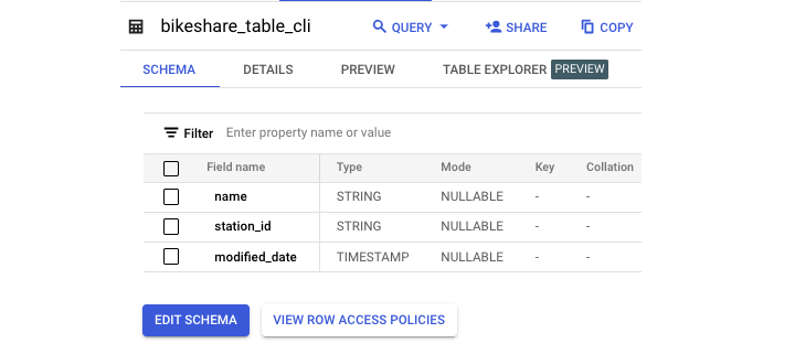
This is the DML to drop sale_id −

Here is the resulting schema −

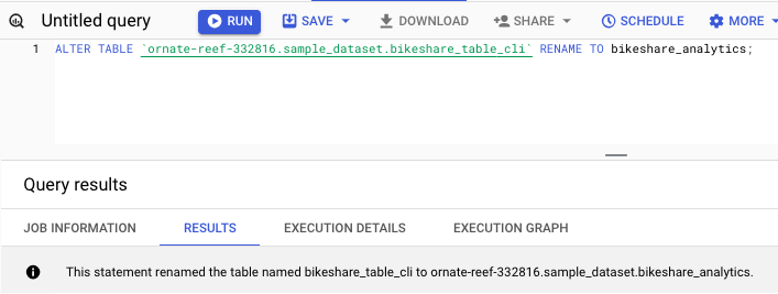
Renaming a Table

You can use the following command to rename a table −

Add a Table Description

Use the following query to add a table description −

You can see in the following screenshot that this statement successfully added a description to the table.

Add Partition Expiration Days

Use the following query to add partition expiration days −

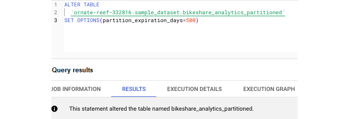
Unlike SELECT statements, any SQL code beginning with ALTER will fundamentally change the structure or metadata of a given table.

Note − You should use these queries with utmost caution.

BigQuery - Copy Table

SQL tables can be copied or deleted as needed in the same way as a file on a desktop.

Copying a table can take two forms −

• Copying / recreating a table
• Cloning a table

Let's find out how cloning a table is different from copying a table.

Cloning a Table in BigQuery

Making a perfect copy of an existing table in BigQuery is known as cloning a table. This task can be accomplished through either the BigQuery Studio UI or through the SQL copy process.

In either case, it is important to keep in mind that any new table created, even if it is a cloned table, will still incur long-term storage and usage charges.

Copying a Table in BigQuery

Copying a table preserves all its current attributes including −

• All data stored
• Partitioning specs
• Clustering specs
• Metadata like descriptions
• Sensitive data protection policy tags

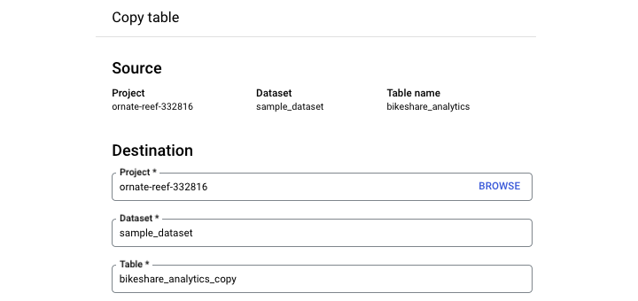
To copy a table in the BigQuery Studio UI, navigate to the query environment. Click on the table you'd like to copy. Select "copy."

It's important to note that this copying process isn't automatic. When you click "copy", you'll need to specify what dataset you're copying the new table to and provide a new table name.

Note − The default naming convention is for GCP to append "_copy" to the end of your original table name.

BigQuery does not support the "SQL COPY" command. Instead, developers can copy a table using several different methods.

Create or Replace Table

Often considered the default create table statement within BigQuery, CREATE OR REPLACE TABLE can double as a de-facto COPY.

CREATE OR REPLACE TABLE project.dataset.table

It's required to supply some kind of query using an AS keyword −

CREATE OR REPLACE TABLE project.dataset.table AS (
)

To perform a copy, you could simply "SELECT * from" an existing table.

In order to create a perfect clone, developers can use the "CREATE TABLE CLONE" keyword. This command creates a perfect copy of an existing table without needing to provide a query.

Between the UI and supported SQL syntax, BigQuery offers flexibility related to copying and cloning tables.

BigQuery - Delete and Recover Table

Deleting a table provides the same two options: UI and SQL syntax. To delete a table in the UI, simply select the table you want to delete and choose "delete table". Since this is a permanent operation, you'll be prompted to type the table name prior to deletion.

Note − You can also DROP a table within the SQL environment.

To delete just the contents of a table and retain the data within, you can use the DELETE command which requires a WHERE clause.

To delete anything without parameters, you can use the following query −

DELETE FROM project.dataset.table
WHERE 1=1

Note − Use this query with extreme caution.

Recovering a Table in BigQuery

Despite the two-step deletion process, it is still very possible to accidentally DROP or delete a table. Consequently, the creators of BigQuery realized that there might be a need to provide users a way to recover tables that were prematurely deleted.

BigQuery Table Snapshots

It's not obvious while you are creating and working with tables in a SQL environment, but in the background, BigQuery is auto-saving your work to an extent.

BigQuery uses "snapshots" to periodically save tables as a way of providing an immediate backup, should the need arise. It's important to note that if a user restores a table from a snapshot they're not actually restoring their original table they're simply restoring to the snapshot or copy of the table.

This tool is not without constraints. BigQuery table snapshots only last 7 days. Therefore, it is only possible to restore a deleted table within 7 days of the initial deletion.

Two Ways to Recover a Table

BigQuery provides two ways to recover a table. Incidentally, neither of them use BigQuery SQL. They require accessing BigQuery through either the gcloud command line or programmatically by accessing the API. Either statement will hinge on selecting the correct timestamp of the snapshot to restore to.

1. Gcloud Command

Here, the command "bq cp" is "bq copy". "No-clobber" is a parameter that will instruct the command to fail if a destination table does not already exist.

bq cp \
 restore \ 
 no-clobber \
snapshot_project_id.snapshot_dataset_id.snapshot_table_id \ 
target_project_id.target_dataset_id.target_table_id

2. Python Function

Ideally, developers will implement precautions to avoid the need for restoration. However, should the worst happen, BigQuery provides this fail-safe.

BigQuery - Populate Table

When first learning BigQuery, one of the quickest ways to immediately use its functions and write SQL queries is to provide an existing data source. One of the easiest data sources to upload and begin working with is a static file.

File Types Accepted in BigQuery

BigQuery considers any table created from a file as an external table.

BigQuery accepts file inputs from either a local upload or cloud storage within GCP's Google Cloud Storage.

File types accepted include −

• CSV (comma separated value)
• JSONL (newline delimited JSON)
• Parquet
• Avro
• ORC

Just like creating an empty table, to populate data, it is necessary to specify a schema. As a reminder, the schema can either be inferred (auto-generated) or provided in the UI or as a JSON file.

Check if BigQuery Supports the Data Types

One of the challenges of working with external files, especially CSVs, is that BigQuery is particular about certain data types.

Before uploading a file, it is a good idea to check BigQuery supports the data types and adjust the input accordingly. For example, BigQuery is very particular about how it ingests timestamp data, preferring that each value have two integers rather than one, even for abbreviated dates.

How does BigQuery Avoid File Upload Errors?

Another challenge developers encounter when loading a file into any SQL table is the presence of special characters, like the newline character "\n." While it is always wise to remove these characters and sufficiently clean the data programmatically, BigQuery provides ways to filter out or entirely ignore lines that may result in a file upload error.

• First, BigQuery allows developers to specify an integer value representing how many errors to allow. This can be helpful if there is one particular bad row that doesn't contain any consequential data.
• Additionally, BigQuery provides a parameter for skipping header rows, including quoted newlines and allowing jagged or malformed rows.

Unfortunately, even with these options, the only way to determine if a file will upload is a bit of trial, error and iteration.

BigQuery Studio: Populate a Table from a SQL Statement

Depending on the situation, there are two ways to populate a table from "scratch", a.k.a. a simple SQL statement.

1. The CREATE OR REPLACE Command

The first, CREATE OR REPLACE, has already been covered. In this case, a developer is creating an entirely new table and must define the table schema in addition to the table content. Typically CREATE OR REPLACE is best used when aggregating or expanding upon data that already exists in a SQL table.

2. The INSERT Command

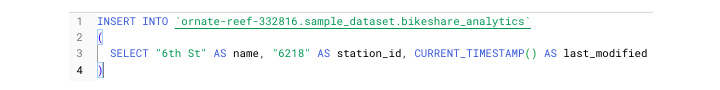
If you find yourself with the "shell" of a table, including a well-defined schema but no data added yet and you don't have a source like an external file or an API payload, then the way you add data is through the INSERT command.

In this case, to properly use INSERT, it's necessary to not just define the columns, types and modes, but also to provide the data being inserted.

Defining data within the confines of SQL involves supplying the value and column alias. For instance −

3. The UNION Command

To add more than one row, use the UNION command. For those unfamiliar with UNION, it is similar to Pandas' concat and essentially "stacks" row entries on top of one another as opposed to joining on a common key.

There are two kinds of UNIONs −

• UNION ALL
• UNION DISTINCT

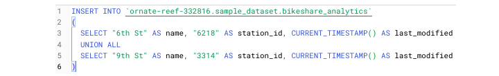
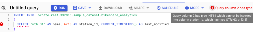
To ensure your data is properly inserted using UNION, it's necessary to ensure that data types agree with each other. For instance, since I provided a STRING value for station_id, I couldn't then change the type to an INTEGER for the following rows.

In professional environments, INSERT is not used to insert one row at a time. Instead, INSERT is commonly used to insert partitions of data, typically by date, i.e., the most recent day's data.

Populate a Table from a Connected Sheet

As is evident by now, querying in BigQuery is different from writing SQL in a local environment due in part to the ability of developers to synchronize BigQuery data with GCP's cloud-based tools. One of the most powerful and intuitive integrations is using BigQuery in combination with Google Sheets.

Exploring the dropdown of external table sources will reveal "Sheets" as a source developers can use to populate a table with data.

Google Sheet as a Primary Data Source

The reason using a Google Sheet as a primary data source is so useful is because, unlike a static CSV, Sheets are dynamic entities. This means that any changes made to the rows within the connected sheet will be reflected in the associated BigQuery tableall in real-time.

To connect a Google Sheet to a BigQuery table, follow the original create table process. Instead of selecting Create Table from Upload, you'll need to select "Drive" as the source. Even though Google Sheets are created in the Sheets UI, they live in Google Drive.

Like CSVs, connected sheets must have defined headers. However, unlike CSVs, developers can specify which columns to include and omit.

The syntax is similar to creating and executing Excel formulas. Simply write the column letter and row number. To select all rows after a given row, preface your column with an exclamation point.

Like: !A2:M

Using the same syntax, you can even select different tabs within a provided sheet. For example −

"Sheet2 !A2:M" 

Like working with CSVs, you can specify which rows and headers to ignore and whether to allow quoted new lines or jagged rows.

An Important Caveat

DML statements like INSERT or DROP do not work on connected sheets. To omit a column, you would need to hide it in your sheet or specify this in your initial configuration.

BigQuery Standard SQL vs Legacy SQL

While SQL doesn't have underlying dependencies like Python (or any other scripting language), there are differences in the BigQuery SQL version you choose.

Since Google Cloud Platform recognizes that developers are familiar with different dialects of SQL, they have provided options for those who may be accustomed to working with a more traditional or "legacy" SQL version.

Difference Between Standard SQL and Legacy SQL

The main difference between standard SQL and legacy SQL is the mapping of types. While legacy SQL supports types that align more closely with universal data types, standard SQL types are more specific to BigQuery. For instance, BigQuery standard SQL supports a much narrower range for timestamp values.

Other differences include −

• Using backticks rather than brackets to escape special characters.
• Table references use colons rather than dots.
• Wildcard operators are not supported.

Toggling between standard and legacy SQL within the BigQuery SQL environment is easy. Before writing and executing your SQL query, simply add a comment: "#legacy" on line 1.

Standard SQL Advantages of BigQuery

Standard SQL empowers SQL developers to write queries with more flexibility and efficiency than the derivative legacy SQL dialect. Standard SQL offers more "real world" utility by providing functions and frameworks that are helpful when dealing with the "messy" data one would encounter in a professional environment.

Standard SQL facilitates the following −

• A more flexible WITH clause which enables users to reuse subqueries and CTEs multiple times within a script.
• User-defined functions that can be written in either SQL or JavaScript.
• Subqueries in the SELECT clause.
• Correlated subqueries.
• Complex data types (ARRAY & STRUCT types).

Incompatibility Between Standard and Legacy SQL

Generally, there won't be many situations in which incompatibility between standard and legacy SQL operations will cause issues. However, there is one scenario that is applicable to AirFlow users.

If using the BigQueryExecuteQuery operator, it is possible to specify whether or not to use legacy SQL. To use standard SQL, set "use_legacy_sql = FALSE".

However, if a developer fails to do this and uses a function only compatible with standard SQL, like TIMESTAMP_MILLIS() (a timestamp conversion function), it is possible that the entire query will fail.

BigQuery - Write First Query

It is possible to open a blank page within the query editor, however it is better to compose your first query directly from the table selection step to avoid syntax errors.

To write your first query in this way, begin by navigating to the dataset that contains the table you'd like to query. Click on "view table." In the upper panel, select "query." Following this process will open a new window in which the table name is already populated, along with any limitations the creator added.

For instance, a table may require a WHERE clause or a suggested query may limit a user to say 1000 rows. In order to follow best practices, replace the " * " with the name of the columns you'd like to query.

• Be mindful of including a GROUP BY clause if adding any aggregations to your SELECT
• If you'd like to be extra vigilant about syntax errors, you can also select column names from the provided schema by clicking on them.

If you follow these steps, you shouldn't have a need to write the table name. However, to get in the habit of formulating correct table references, remember the formula is: project.dataset.table. These elements are all enclosed in backticks (not quotations).

One unique element of BigQuery Studio is that the IDE will tell you if a query will run or not. This will be indicated by a green checkmark.

Once you've confirmed everything looks correct, hit run. As the query runs you'll see execution metrics like data processed, time it takes the query to run and number of steps required. If you glance at the bottom panel you'll also see the amount of slots it takes to run.

Write Your First Query on Cloud Shell Terminal

Like querying in the UI, querying in the cloud shell terminal follows a similar structure and allows users to use SQL syntax to access and manipulate data.

The "bq" Query and its Common Flags

Writing and executing a query within cloud shell is simple enough with the command bq query. In the same line, users can supply flags that dictate certain aspects of execution.

Some of the more common flags for the bq query command include −

• allow-large-results (does not cancel jobs due to large results)
• batch = {true | false}
• clustering-fields = [ ]
• destination-table = table_name

You may notice that all of these parameters correspond to the drop-down menu that appears when creating a table or running a query within the UI.

To run a query within cloud shell −

• Log into GCP
• Enter the cloud shell terminal
• Authenticate (done automatically)
• Write and execute query

Which looks like −

(ornate-reaf-332816)$ bq query --use_legacy_sql=false \ 'SELECT * FROM 
ornate-reef-332816.sample_dataset.bikeshare_2022_stsore_date';

Results appear as a terminal output. While results are not rendered like BigQuery UI results, the output is still neat and understandable.

BigQuery - CRUD Operations

CRUD, standing for CREATE, REPLACE, UPDATE and DELETE, is a foundational SQL concept. Unlike a conventional query that will simply return data in a temporary table, run a CRUD operation, and a table's structure and schema fundamentally changes.

CREATE OR REPLACE Query

BigQuery combined the C and R of CRUD with its statement CREATE OR REPLACE.

CREATE OR REPLACE can be used with BigQuery's various entities, like −

• Tables
• Views
• User-defined functions (UDFs)

The syntax for using the CREATE OR REPLACE command is −

CREATE OR REPLACE project.dataset.table 

While a create operation will create an entirely new entity, an UPDATE statement will alter records at the row (not table) level.

UPDATE Query

Unlike CREATE OR REPLACE, UPDATE used another bit of syntax, SET. Finally, UPDATE must be used with a WHERE clause so UPDATE knows which records to change.

Put together, it looks like this −

The above query updates the table but only impacts rows where the date is equivalent to the current date. If this is the case, it will change the date to yesterday.

DELETE Command

Like UPDATE, DELETE also requires a WHERE clause. The syntax of DELTE query is simple −

DELETE FROM project.dataset.table
WHERE condition = TRUE 

ALTER Command

In addition to CRUD statements, BigQuery also has the previously covered ALTER statement. As a reminder, ALTER is used to −

• Add columns
• Drop columns
• Rename a table

Use each of these functions with caution, especially when working with production data.

BigQuery - Partitioning & Clustering

Since both "partitioning" and "clustering" have been used in this tutorial already, it's helpful to provide additional context.

What are Partitioning and Clustering?

Both terms are used to describe two methods of optimizing data storage and processing.

Partitioning is how a developer segments data, typically (but not always) by a date element like year, month or day. Clustering describes how data is sorted within the specified partition.

To use either storage method, you must define a desired field. Only one field may be used for partitioning but multiple fields may be used for clustering.

It's important to note that to apply either partitioning or clustering, you must do this at the "create table" stage of your build. Otherwise, you will be required to drop/recreate the table with the updated partitioning/clustering specs.

How to Apply Partitioning or Clustering to a Table

To apply partitioning and/or clustering to a table upon creation, run the following −

You can also specify these directions within the UI. Before hitting "create table", take a moment to fill in the fields found directly below the schema creation box.

If you apply the partitioning / clustering properly, it can significantly reduce both long-term storage cost and processing time, especially when querying a large table.

BigQuery - Data Types

Understanding BigQuery's usage and interpretation of data types is essential when it comes to loading and querying data. As demonstrated in the schema chapter, every column loaded into BigQuery must have a defined, acceptable type.

BigQuery accepts many data types that other SQL dialects use, and also offers data types unique to BigQuery.

Common Data Types Across SQL Dialects

Data types that are common across SQL dialects include −

• STRING
• INTEGER
• FLOAT
• BOOLEAN

BigQuery also facilitates special data types, like JSON arrays, which will be discussed in a later chapter.

Note − If a schema is not provided or a type is not specified during a load process, BigQuery will infer the type. Though, for integrations that rely on unpredictable upstream data, this is not necessarily a positive outcome.

Like partitioning and clustering columns, types must be specified at the time of table creation.

Alter Types Using the CAST() Function

It is possible to alter types (temporarily or permanently) within a query. To do this, use the CAST() function. CAST uses the following syntax −

CAST(column_name AS column_type)

For Instance −

CAST(id AS STRING)

Like specifying the wrong type, trying to force CAST an incompatible type can be frustrating and lead to infrastructure breaks.

For a more proven way to convert types, use SAFE_CAST(), which will return NULL for incompatible rows, instead of breaking entirely −

SAFE_CAST(id AS STRING)

Developing a solid understanding of how BigQuery will interpret a given input's type is essential to creating robust SQL queries.

BigQuery Data Types STRING

Among the most common data types SQL developers work with, STRING types in BigQuery are typically easy to identify. However, there are occasional quirks regarding a string's manipulation or interpretation.

Generally, a string type consists of alphanumeric characters. While a string type can include integer-like digits and symbols, if STRING is the specified type, this information will be stored like a conventional string.

One tricky situation new developers encounter is working with a row that contains an INTEGER or FLOAT value with a symbol, like in the case of currency.

While it might be assumed $5.00 is a FLOAT because of the decimal point, the U.S. dollar sign makes it a string. Therefore, when loading a row with a dollar sign, BigQuery will expect this to be defined in your schema as a STRING type.

DATE Data Type

A subset of the STRING type is the DATE data type.

• Even though BigQuery has its own designation for date values, the date values themselves are represented as strings by default.
• For those who work with Pandas in Python, this is similar to how date fields are represented as objects within a data frame.
• There are a variety of functions dedicated solely to parsing STRING data.

STRING Functions

Notable STRING functions include −

• LOWER() − Converts everything within a string to lowercase
• UPPER() − The inverse of lower; converts values to uppercase
• INITCAP() − Capitalizes only the first letter of each sentence; i.e. sentence case
• CONCAT() − Combines string elements

Importantly, data types in BigQuery default to STRING. In addition to conventional string elements, this also includes lists for which a developer does not specify a REPEATED mode.

INTEGER & FLOAT

Chances are, if you're working with BigQuery on an enterprise (business) scale, you'll work with data involving numbers. This could be anything from attendance data to operating revenue.

In any case, a STRING data type does not make sense for these use cases. This is not just because such numbers don't have a currency symbol like a dollar sign or euro accompanying them, but because, to generate useful insights, it requires utilizing functions specific to numeric data.

Note The distinguishing mark between an INTEGER and FLOAT is simple: "."

In many SQL dialects, when it comes to specifying numeric values, developers are required to tell a SQL engine how many digits to expect. This is where conventional SQL gets designations like BIGINT.

BigQuery encodes FLOAT types as 64-bit entities. This is why, when you CAST() a column to a FLOAT type, you do so like this −

CAST(column_name AS FLOAT64) 

Notable INTEGER and FLOAT Functions

Other notable INTEGER and FLOAT functions include −

• ROUND()
• AVG()
• MAX()
• MIN()

Points to Note

An important caveat of the FLOAT type is that in addition to specifying period separated digits, the FLOAT type is also the default type for NULL.

If using SAFE_CAST(), it may be a good idea to include additional logic to convert any returned NULL values from FLOAT to a desired type.

BigQuery - Complex Data Types

BigQuery, in addition to supporting "regular" data types like STRING, INTEGER and BOOLEAN, also provides support for so-called complex data. Often this is also referred to as nested data, since the data does not fit into a conventionally flat table and must live in a subset of a column.

Complex Data Structures Are Common

Support for nested schemas allows for more streamlined loading processes. Although Google Cloud lists various tutorials regarding the following data types as "advanced", nested data is very common.

Knowing how to flatten and work with these data types is a marketable skill for any SQL-oriented developer.

The reason these data structures are common are because source data, like a JSON output from an API, often returns data in this format −

[{data: "id": '125467", "name": "Acme Inc.", "locations": 
   {"store_no": 4, "employee_count": 15}}]

• Notice how both "id" and "name" are on the same level of reference. These could each be accessed using "data" as a key.
• However, to get fields like "store_no" and "employee_count", it would be necessary to not only access the data key, but also to flatten the "locations" array.

This is where BigQuery's complex data type support is helpful. Instead of a data engineer needing to write a script that would iterate through and unnest "locations", this data could be loaded into a BigQuery table as is.

Complex Data Structures in BigQuery

BigQuery supports the following three types of complex or nested data −

• STRUCT
• ARRAY
• JSON

Strategies for handling these types will be explained in the next chapters.

BigQuery - STRUCT Data Type

STRUCTs and ARRAYs are how developers store nested data within BigQuery's columnar structure.

What is a Struct?

A STRUCT is a collection of fields with a specified type, which is required, and a field name, which is optional. Notably, STRUCT types, unlike ARRAYs, can contain a mixture of data types.

To better understand the STRUCT type, take another look at the example from the previous chapter, now with a few changes.

"locations": [
   {"store_no": 4, "employee_count": 15, "store_name": "New York 5th Ave"}, 
   {"store_no": 5, "employee_count": 30, "store_name": "New York Lower Manh"}
]

While previously "locations" was a dict (expressed in JSON) of the same type, now it contains two STRUCTs which have a type of <INTEGER, INTEGER, STRING>.

• Despite supporting a STRUCT type, BigQuery does not have an explicit label STRUCT available during the table creation stage.
• Instead, a STRUCT is indicated as a RECORD with a NULLABLE mode.

Note − Think of a STRUCT as more of a container than a dedicated data type.

When defined in a schema, the elements inside the STRUCT will be represented and selected with a "." Here, the schema would be −

{"locations", "RECORD", "NULLABLE"},
{"locations.store_no", "INTEGER", "NULLABLE},
{"locations.employee_count", "INTEGER", "NULLABLE"},
{"locations.store_name", "STRING", "NULLABLE"}

dot Notation

To select a STRUCT element, it is necessary to use the dot notation in the FROM clause −

When the query gets executed, you may get an output like this −

BigQuery - ARRAY Data Type

Unlike a STRUCT type, which is allowed to contain data of differing types, an ARRAY data type must contain elements of the same type.

• In programming languages like Python, an ARRAY (also known as a list) is represented with brackets: [ ].
• STRUCT types can contain other structs (to create very nested data), an ARRAY may not contain another ARRAY.
• However, an ARRAY can contain a STRUCT, so a developer could encounter an ARRAY with several STRUCTs embedded within.

BigQuery will not label a column as an explicit ARRAY type. Instead, it is represented with a different mode. While a regular STRING type has a "NULLABLE" mode, the ARRAY type has a "REPEATED" mode.

STRUCT types can be selected using a dot, however ARRAY types are more limited when it comes to surface-level manipulation.

It is possible to select an ARRAY as a grouped element:

However, selecting an element of an array using a dot or any other method is impossible, so this wouldn't work −

The UNNEST() Function

To access names from within store_information, it is necessary to perform an extra step: UNNEST(), a function which will flatten the data so it is more accessible.

The UNNEST() function is used in the FROM clause with a comma. For context: The comma represents an implicit CROSS JOIN.

To properly access this ARRAY, use the following query −

It will fetch you an output table like this −

In addition to using UNNEST(), it's also possible to alias the record. The resulting alias, "wd", can then be used to access the unnested data.

BigQuery - JSON Data Type

JSON is the newest data type the BigQuery supports. Unlike the STRUCT and ARRAY types, JSON is relatively easy to recognize.

For developers who have worked with data in a scripting language or those who have parsed API responses, JSON data will be familiar.

JSON data is indicated by curly brackets: { }, like a Python dictionary.

Note − Prior to BigQuery introducing support for the JSON type, JSON objects would need to be represented as a STRING with a NULLABLE mode.

Developers can specify JSON in both the UI and in text-based schema definitions −

Not storing JSON data as a JSON type won't necessarily result in a failed load, because BigQuery can support the STRING type for JSON data.

However, not storing JSON data properly means that developers lose access to powerful JSON-specific functions.

Powerful JSON Functions

Thanks to built-in functions, developers working with JSON data in BigQuery don't need to write scripts to flatten JSON data. Instead, they can use JSON_EXTRACT to extract the contents of a JSON object, which then allows for the handling and manipulation of the resulting data.

Other powerful JSON functions include −

• JSON_EXTRACT_ARRAY()
• PARSE_JSON()
• TO_JSON()

Being able to accurately and intuitively query JSON data within BigQuery saves developers from needing to use complex CASE logic or write custom functions to extract valuable data.

BigQuery - Table Metadata

While being able to analyze and understand the scope and content of organizational data is important, it is also essential for SQL developers to understand aspects of performance and storage cost using BigQuery.

This is when querying BigQuery table metadata can be useful for developers and invaluable for organizations seeking to leverage the SQL engine to its fullest extent.

For those who have not worked extensively with metadata: Metadata is, as the name implies, data about data. Typically this relates to statistics surrounding things like resource performance or monitoring.

BigQuery offers several metadata stores that users can query to better understand how their project consumes resources, some of which include the following −

• INFORMATION_SCHEMA
• __TABLES__ view
• BigQuery audit logs

Each of these tables can be queried in the same way as stored data.

For both the INFORMATION_SCHEMA and __TABLES__ it is helpful to note there is a different syntax regarding the table reference.

Instead of following the typical: project.dataset.table notation, both INFORMATION_SCHEMA and __TABLES__ have elements that are referenced following the closing backtick.

INFORMATION_SCHEMA is a data source that has several offshoot resources like COLUMNS or JOBS_BY_PROJECT

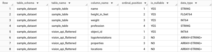
For instance, referencing the INFORMATION_SCHEMA looks like this −

It will fetch the following output −

TABLES View

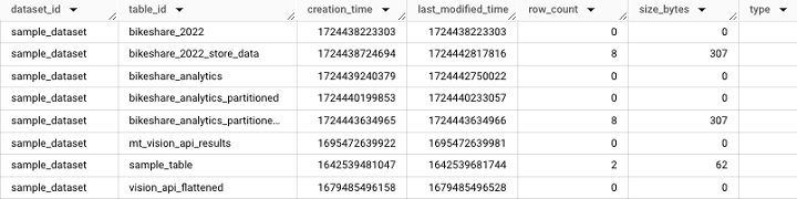
The TABLES view provides information at a table-level, such as table creation time and the user who last accessed the table. It is important to note that the TABLES view is accessible at the dataset level.

It will fetch the following output −

Creating a Schema Based on an Existing Table

One helpful use case for INFORMATION_SCHEMA.COLUMNS is the ability to create a schema based on an existing table using this query −

BigQuery - User-defined Functions

One of the advantages of BigQuery is the ability to create custom logic to manipulate data. In programming languages like Python, developers can easily write and define functions that can be utilized in multiple places within a script.

Persistent User-defined Functions in BigQuery

Many SQL dialects, including BigQuery, support these functions. BigQuery calls them persistent user-defined functions. They're either UDFs (user-defined functions) or PUDFs (persistent user-defined functions) for short.

The essence of user-defined functions can be broken into two steps −

• Defining function logic
• Employing a function within a script

Defining a User-defined Function

Defining a user-defined function begins with a familiar CRUD statement: CREATE OR REPLACE.

Here, instead of CREATE OR REPLACE TABLE, it is necessary to use CREATE OR REPLACE FUNCTION followed by the AS() command.

Unlike other SQL queries that can be written within BigQuery, when creating a UDF, specifying an input field and type is required.

These inputs are defined in a similar way to a Python function −

(column_name, type)

To see these steps put together, I've created a simple temporary UDF, specified by TEMP FUNCTION that parses various URLs based on user input.

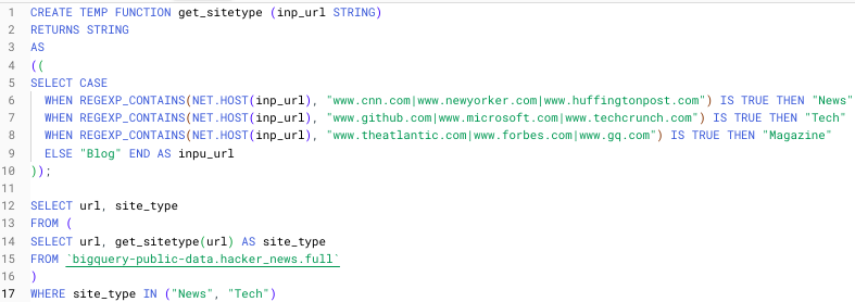
The steps to create the above temporary function are −

• CREATE TEMP FUNCTION
• Specify function name (get_sitetype)
• Specify function input and type (inp_url, STRING)
• Tell the function what type to return (STRING)

The REGEXP_CONTAINS() function searches for a match on strings that contain the URL strings provided. The NET.HOST() function extracts the host domain from the input URL string.

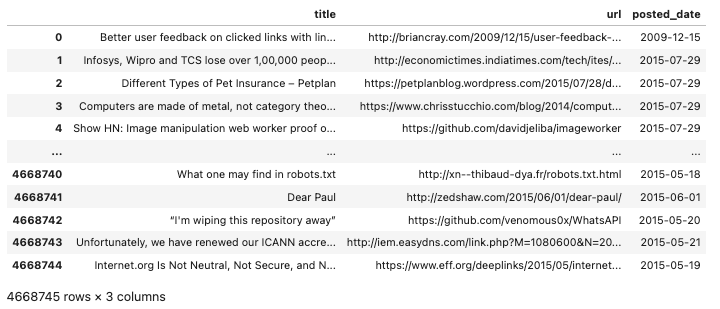
Applying this to the hacker news dataset (a BigQuery public dataset), we can generate an output that classifies the stored URLs into different categories of media −

Note − Temporary functions must be immediately followed by a query.

BigQuery - Connecting to External Sources

While the majority of the tutorial, up to this point, has concerned the UI and the cloud terminal, it's time to explore connecting to BigQuery through external sources.

Limitations of Writing Queries in the UI

Even though it may be convenient to write queries in BigQuery Studio, the truth is, this only fulfills a limited range of purposes −

• Initially developing a SQL query or script
• Debugging a query
• Conducting spot checks or quality assurance

Simply writing and running queries in the UI doesn't help deliver automated data solutions. This means that in the BigQuery SQL environment, you can't −

• Access the BigQuery API
• Integrate with Airflow
• Create ETL pipelines

External BigQuery Integrations

In the following chapters, we'll explore how to integrate BigQuery with −

• BigQuery Scheduled Queries
• BigQuery API (Python)
• Cloud Composer / Airflow
• Google Sheets
• BigQuery Data Transfers

External BigQuery integrations empower developers to leverage the power of SQL to perform the following tasks −

• Create automated extract load (EL)
• Extract transform load (ETL)
• Extract load transform (ELT) jobs

BigQuery - Integrate Scheduled Queries

Scheduled queries, in addition to being the most intuitive external integration with BigQuery (external because the mechanism relies upon the BigQuery Data Transfer service), can be scheduled from BigQuery Studio.

If you prefer, you can also navigate to "Scheduled Queries" on the sidebar. However, even this page will prompt you to "Create Query" which will take you back to the UI. So, it's best to create and schedule your query from the UI by −

• Compose query in the SQL workspace.
• Validate and run the query (a query will only run or be scheduled if it is valid).
• Choose "Schedule Query" which will open up a drop-down menu.

Once in the "Schedule Query" menu, you must fill in −

• Name of the query
• Schedule frequency
• Start time
• End time

If you don't fill in an end time, the query will run on its assigned schedule in perpetuity.

Note − One caveat about scheduled queries is that once they are scheduled, there are certain aspects of the query run parameters (like the user associated with the query) that cannot be changed in the UI.

For this, it is necessary to access scheduled queries either via the BigQuery API or command line.

Integrate BigQuery API

The BigQuery API allows developers to leverage the power of BigQuery's processing and Google SQL data manipulation functions for recurring tasks.

The BigQuery API is a REST API and supports the following languages −

• C#
• Go
• Java
• js
• PHP
• Python
• Ruby

Since Python is one of the most popular languages for data science and data analysis, this chapter will explore the BigQuery API within the context of Python.

BigQuery API Deployment Options

Just like developers can't deploy SQL directly from BigQuery Studio, for production workflows, code that accesses the BigQuery API must be deployed through a relevant GCP product.

Deployment options include −

• Cloud Run
• Cloud Functions
• Virtual Machines
• Cloud Composer (Airflow)

BigQuery API Requires Authentication

Using the BigQuery API requires authentication −

• If running a script locally, it's possible to download a credential file associated with the service account running BigQuery and then setting that file as an environment variable.
• If running BigQuery in a context connected to the cloud, like in a Vertex AI notebook, authentication is done automatically.

To avoid downloading a file, GCP also supports Oauth2 authentication flows for most applications.

Once authenticated, typical BigQuery API use cases include −

• Running a SQL script containing a CRUD operation for a given table.
• Retrieving project or dataset metadata to create monitoring frameworks.
• Running a SQL query to synthesize or enrich BigQuery data with data from another source.

The ".query()" Method

Undoubtedly, one of the most popular BigQuery API methods is the ".query() method". When paired with Pandas' .to_dataframe(), it presents a powerful option for querying and displaying data in a readable form.

This query should fetch the following output −

The BigQuery API isn't a black box. In addition to logging (using a Google Cloud Logging client), developers can see real-time job information broken down at both a personal user and project level in the UI. To troubleshoot any failed jobs, this should be your first stop.

BigQuery - Integrate Airflow

Running a Python script to load a BigQuery table can be helpful for an individual job. However, when a developer needs to create several sequential tasks, isolated solutions aren't optimal. Therefore, it is necessary to think beyond simple execution. Orchestration is required.

BigQuery can be integrated with several popular orchestration solutions like Airflow and DBT. However, this tutorial will highlight Airflow.

Directed Acrylic Graphs (DAG)

Apache Airflow allows developers to create execution blocks called Directed Acrylic Graphs (DAG). Each DAG is comprised of many tasks.

Each task requires an operator. There are two important BigQuery-compatible operators −

• BigQueryCheck Operator
• BigQueryExecuteQuery Operator

BigQueryCheck Operator

The BigQueryCheckOperator allows developers to conduct upstream checks to determine whether or not data has been updated for the day.

If the table does not have an upload timestamp included in its schema, it is possible to query metadata (as discussed earlier).

Developers can determine the time a table was last updated by running a version of this query −

BigQueryExecuteQuery Operator

To execute SQL scripts that depend on upstream data, SQL developers can use the BigQueryExecuteQuery operator to create a load job.

A deeper explanation of Airflow is beyond the scope of this tutorial, but GCP provides extensive documentation for those who would like to learn more.

BigQuery - Integrate Connected Sheets

For those opting to use a cloud service like BigQuery as a data warehouse, it is often a goal to migrate data from spreadsheets to a database. Consequently, pairing a data warehouse and a spreadsheet may seem redundant.

However, connecting a Google Sheet to BigQuery allows for a seamless recurring "refresh" of spreadsheet data, since the source is a view or table in BigQuery.

Google Sheets supports BigQuery integration in two ways −

• Connecting directly to a table.
• Connecting to the result of a custom query.

Unlike BigQuery where available external data sources are presented in a drop-down menu, finding data sources in Google Sheets requires a bit of digging.

Connecting a BigQuery Resource to Google Sheets

To connect a BigQuery resource to Google Sheets, follow the steps given below −

• Open a new Google Sheet
• Click on the "data" tab
• Under data, navigate to data connections
• Choose an existing dataset
• Find your desired table
• Alternatively, write a custom query
• Click connect

The sheet should change from a standard spreadsheet into a UI that resembles a hybrid between a spreadsheet and SQL table.

How to Ensure Synchronization and Schedule a Refresh?

While following these steps ensures the connection is live, stopping here will not ensure future synchronization.

• To automatically update the sheet as its associated resource is updated, you must schedule a refresh.
• You can schedule a refresh by navigating to "Connection Settings."
• Like configuring a scheduled query, scheduling a refresh is simple. Choose your refresh interval, start time and end time.

Once configured, the sheet will now update on that schedule, assuming data is available in the BigQuery table.

BigQuery - Integrate Data Transfers

BigQuery Data Transfers facilitate syncs of data from Google-affiliated products and funnel the resulting payload into BigQuery. Since these data transfers are between Google products, they are based on out-of-the-box reports.

During configuration, users have the option of choosing the report they would like to import. This, unfortunately, means there is no room for upstream customization.

While it might be intuitive to worry about a given report not having a specific field, the opposite is often true. Google's reports often contain so much data that it is necessary to construct views to extract only information that is relevant to your use case.

Data Transfers Require Authentication

Like other BigQuery integrations, data transfers require authentication.

• Luckily, since the transfer is initially configured in the UI, it is a simple auth flow.
• Using Oauth2, a user setting up a BigQuery transfer is required to log into and verify the account connected to Google Cloud Platform.
• Once authenticated, developers can choose from a drop-down of Google products and report types.

One of the most important aspects of the process, to facilitate ease of use with the resulting data, is to provide a memorable name as the suffix of the resulting table.

Note − There are certain reports like billing reports that do not allow users to change the name of the ingested tables.

Examples of Reports

Examples of reports that can be scheduled as Data Transfers include −

• DFP
• Google Ad Manager
• YouTube Channel Reports

These out-of-the-box reports can remove the development burden for certain BigQuery-compatible data resources.

BigQuery - Materialized View

In addition to the creation of tables and views, BigQuery also facilitates the creation of materialized views.

What is a Materialized View?

A materialized view is similar to a table in that it is a "snapshot" of data. However, the materialized view differs in that a true materialized view will update dynamicallyall without needing to run a query.

Types of Materialized Views

Broadly, there are two kinds of materialized views −

• A view that has been saved as a table and will be updated on a recurring basis from an outside source.
• A "true" materialized view created in BigQuery Studio.

Here is example architecture for the first kind of view −

• SQL queries an existing view
• Within a Python script, that view is converted to a dataframe
• The dataframe is uploaded to BigQuery
• The materialized view is either appended to or overwritten

Since the above outlined a multi-step process, BigQuery has streamlined the creation and maintenance of materialized views.

Creating a BigQuery Materialized View

Users can create a BigQuery materialized view by running the CREATE MATERIALIZED VIEW SQL statement followed by −

• Project
• Dataset
• New mv name
• SQL statement

Example

Here's an example in which an existing table with hypothetical sales data is materialized −

Note the following limitations, per BigQuery documentation −

• Each table is limited to 20 materialized views within a dataset
• There can only be 100 materialized views within a project
• There can only be 500 materialized views within an organization

Write a Simple SQL Script in BigQuery

Putting everything together now, it's time to write a simple script that will −

• Utilize dynamic variables
• DELETE yesterday's data
• INSERT new data into a table
• Use a query to select/load data

One area not covered so far is how to define and use variables within a SQL script.

In BigQuery, variable syntax is as follows −

DECLARE variable_name TYPE DEFAULT function used to create dynamic variable

As an example −

DECLARE yesterday DATE DEFAULT DATE_SUB(CURRENT_DATE(), INTERVAL 1 DAY)

And this is how we'll begin the following script, which deletes previous data from the Austin bike share partitioned table and inserts only the most recent data.

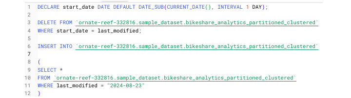
When running this in BigQuery, the SQL engine will run this in stages due to the semicolon. The final results can be seen by clicking "View results."

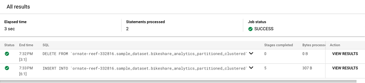
Clicking on "View results" generates this output.

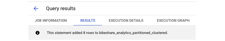
And, finally, we can see the new rows added to the table.

BigQuery - Roles & Permissions

Running a query within the BigQuery Studio UI is deceptively seamless. Since a developer is signed into their Google Cloud Platform account, there is no need to authenticate. However, behind the scenes, certain restrictions and guardrails assure developers are only able to take certain actions within a project.

Identity Access and Management (IAM) Roles

These restrictions or designations are known as roles and permissions. Within GCP, these are known as Identity Access and Management (IAM) roles.

Broadly, these roles fit into 3 tiers −

• BigQuery Admin
• BigQuery Data Editor
• BigQuery User

1. BigQuery Admin

BigQuery admins can do anything within a project such as create or delete tables and start and stop jobs from runningeven those initiated by other users.

2. BigQuery Data Editor

A BigQuery data editor has slightly fewer permissions. While they can read, update and delete tables or views, they lack control and authority at a project level and cannot exert control over other users' jobs.

3. BigQuery User

BigQuery users are the lowest tier of BigQuery IAM roles. They are extremely limited when it comes to accessing and manipulating resources. Among their limited abilities: Listing tables and accessing metadata.

Playing with BigQuery on your own won't necessitate knowledge of any of these roles or permissions. However, as you work with enterprise-scale data, understanding the roles and permissions can help accelerate solutions to access issues or come in handy when provisioning service accounts.

BigQuery: Policy Tags & PII

Just like BigQuery admins can grant permissions to and exert influence over users with lower-level access, they can also control what data individuals can see and interact with. This can be accomplished using policy tags.

What are Policy Tags?

A policy tag is essentially a censor bar for an organization's data. Admins can apply this tag to block users within the organization from accessing sensitive data. While some aspect of determining what constitutes sensitive data is subjective, there is also an objective definition.

What is Personally Identifiable Information (PII)?

In data governance, sensitive data is known as Personally Identifiable Information (PII). PII includes any attribute that can be used to immediately and intimately identify a given individual. It includes the following information −

• Phone number
• Biometric information
• Email
• Social security number (US)
• Credit card numbers

Any of the above is considered to be extremely sensitive information that must be carefully guarded. To guide protection, GCP has identified 150+ PII attributes in documentation for its data governance product, Data Loss Prevention.

Policy Tags can be Configured

Policy tags can also be issued to protect an organization against internal users who shouldn't have access to business-critical information like revenue data.

Policy tags can be configured and then applied in BigQuery by −

• Selecting a table
• Hitting "edit schema"
• Selecting all columns that may contain sensitive information
• Applying configured policy tag

Developers can tell when such a tag has been applied because it will appear as a gray box next to a field name in a table's schema.

BigQuery - Query Optimization

BigQuery is powered by cloud computing, however it does not imply that compute power is infinite. It also does not mean that every query will run for the exact same length of time, no matter the time of day or how many processes are competing for slots.

What is Query Optimization?

Optimization is a buzzword that gets used often by those in data engineering and other programming disciplines.

With SQL, optimization comes in two forms −

• Code-based Optimization
• Platform-based Optimization

Code-based optimization is complex to conceptualize and execute. Therefore, it is beyond the scope of this tutorial. Instead, we will focus on tools within BigQuery that enable users to accurately track and actively curb over usage.

Through increased visibility and creative slot allocation, it is possible to maintain a BigQuery project with multiple users and have adequate storage and slot space for all. This is achieved through −

• Tracking usage through execution graphs and data lineage tools.
• Running queries in different modes to lessen the amount of data processed at a given time.
• Leveraging tools like BI Engine to segment repeat offenders (tables) to proactively limit the scope of data processed during high-volume traffic hours.

Batch vs. Interactive Modes

Upon writing your first few queries in the BigQuery Studio SQL environment, it may seem like all queries run in the same way. And, in a sense, you're correct. All queries utilize a certain amount of slots which is expressed in slot hours during execution. However, there are actually two different ways to run BigQuery queries to conserve both processing and costs.

The majority of BigQuery queries are executed in what is called interactive mode. In fact, this is the default execution state for BigQuery queries. And the UI doesn't make the ability to change modes visible or obvious. To view or change a query's execution mode requires navigating to query settings.

Once in that view, you can configure your next query run. In addition to selecting a query mode, developers also have the option to choose how to save a query's results, being presented with options ranging from a temporary table, a new BigQuery table or overwriting an existing table's contents. Below these options is the menu for selecting batch vs. interactive.

While interactive mode executes queries instantly, batch mode allows users to −

• Queue desired BigQuery jobs.
• Run lower-priority queries without impacting higher-priority jobs (that likely consume more resources).

Running a batch mode job helps users circumvent a BigQuery query execution restriction: Users can run, at most, 20 concurrent queries.

If a batch job is competing with an in-progress interactive job for slots, the batch job will be put on hold or "queued" until space is available. This helps both conserve resources and avoid hitting the hard rate limits imposed on interactive queries.

BigQuery - BI Engine

In addition to optimization settings within BigQuery, BigQuery also offers a concurrent service, BI Engine, whose purpose is to scan and optimize BigQuery query performance.

• BI Engine is an in-memory service that analyzes the scope of job being run versus the amount of slots and compute resources available at the time of execution.
• Not only does BI Engine analyze query resources, it actively accelerates their execution (hence the "engine") after allocating the available resources.
• BI Engine is configurable and customizable, meaning that developers can choose which tables and views to include within its scope.
• BI Engine is a product within BigQuery. To reach the BI landing page, simply search "BI Engine" in the Cloud Console search bar.

The BI Engine page will prompt you to Create a Reservation.

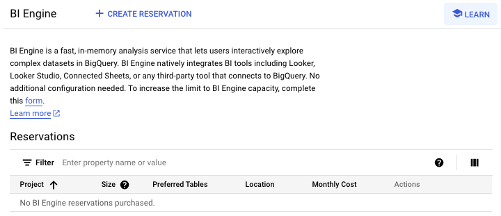
Once you click on "Create a Reservation", you'll be able to configure how many gigabytes you would like to set within the scope of BI Engine and add the tables you would like to include within the scope of BI Engine's performance optimization capabilities.

Query Acceleration of BI Engine

Additionally, BI Engine syncs with the BigQuery API to provide query acceleration benefits to tables loaded, updated or modified from automated processes.

BI Engine's crowning achievement is vectorized runtime, which allows it to leverage cloud CPUs and enables it to compress data for seamless runs.

The real power of BI Engine lies in its ability to integrate with BigQuery-adjacent platforms and applications. For instance, a Looker dashboard that creates data based on BigQuery queries would be eligible for BI Engine acceleration.

Use Cases of BI Engine

BI Engine would most benefit a user with high-volume data tables that are queried routinely.

BI Engine use cases include −

• Resource-intensive visualizations powered by BigQuery.
• You have specific large and frequently-queried tables.
• Multiple users who query resources at similar times and cause performance log jams.

Regardless, BI Engine remains a powerful optimization strategy for any user seeking to make processes more efficient and less compute-intensive.

BigQuery - Monitoring Usage & Performance

Understanding usage and performance constraints is critical, especially for those working within an organization. Maintaining constant visibility regarding users and data sources that are consuming disproportionate amounts of slot time can help BigQuery administrators make informed decisions about limiting access to resources and spawn productive conversations among teams who run resource-intensive jobs.

Performance Dashboards

To achieve more transparent real-time monitoring, BigQuery has made performance dashboards available in the monitoring tab within the BigQuery Studio UI.

Note − Performance is charted each time a query is executed.

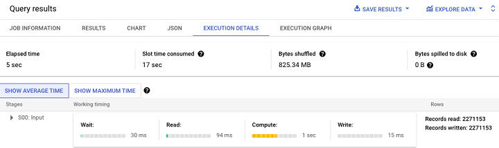
Additionally, BigQuery provides an execution graph for a more visually-friendly interpretation of query performance.

On a project level, administrators can view BigQuery data within the "Monitoring" dashboard. Monitoring is available at project level and dataset level.

Project Level Monitoring

The project level shows how many queries are currently running or "in flight".

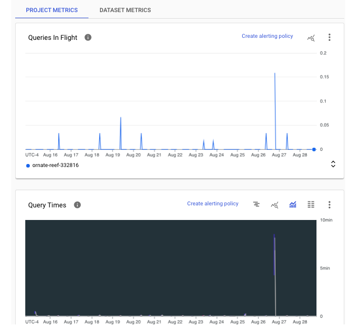
Dataset Level Monitoring

At a dataset level, we can see stored bytes per table.

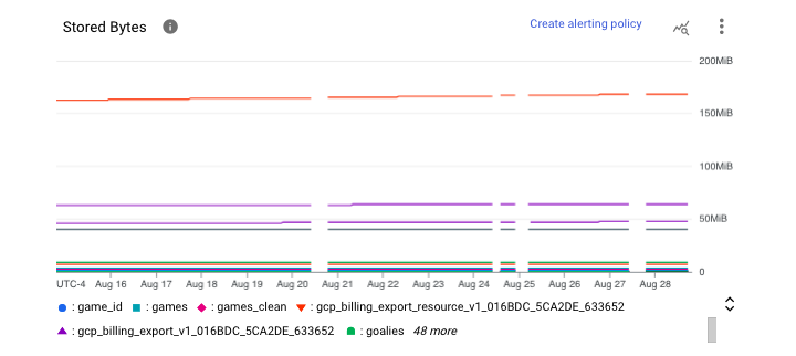
To access and manipulate these charts, follow these steps −

• Navigate to BigQuery
• Select Administration
• Click Monitoring
• If desired: Toggle live data

Within this UI, users can also access Operational Health, which offers information in the form of two different views: A summary view and a more detailed view.

Some top line metrics within Operational Health summary tables that both administrators and users would find helpful include −

• Slot usage
• Shuffle (reservation re-allocation) usage
• Concurrency (simultaneous jobs)
• Bytes processed
• Job duration
• Total storage

Note − Usage units are bytes (can be converted to gigabytes or terabytes if necessary).

For a more granular view, users can query the INFORMATION_SCHEMA views using the metadata query techniques from earlier in this tutorial.

Common Errors of BigQuery

Despite being armed with education and information regarding BigQuery features, like any development process, errors are possible and, in fact, are likely inevitable. New users are particularly susceptible to BigQuery errors given their inexperience with the platform.

Types of BigQuery Errors

BigQuery errors present in two categories −

• Code-based errors
• Platform-based errors

Although BigQuery's SQL dialect (Google SQL) is intended to be universally understood and reminiscent of other SQL dialects, syntax errors can occur and, frankly, can be quite frustrating.

BigQuery Syntax Errors

Here is a non-exhaustive list of BigQuery syntax mistakes −

• Using apostrophes instead of backticks.
• Omitting either the dataset or table in a FROM clause.
• Using UNNEST() incorrectly (on a STRUCT instead of an ARRAY).
• Forgetting a GROUP BY clause when using an aggregate function like AVG().
• Forgetting a comma between column names.

Platform-based Errors

Platform-based errors stem from misunderstanding BigQuery's execution constraints and may include −

• Running more than 20 concurrent queries.
• Not writing the results of a large query to a table resulting in a "result too large" error.
• Not running a large query as a batch job.
• Overwriting or truncating a table instead of appending a result.

Unfortunately, it is impossible to flag nearly every error a new BigQuery SQL developer will encounter. However, the above represent a broad variety of issues you may encounter.

BigQuery - Data Warehouse

For many organizations, BigQuery is a natural candidate for a data warehouse. A data warehouse is a business system and central repository to store data for analysis and then downstream reporting.

Note Typically, data stored within a data warehouse is structured or semi-structured, as opposed to a data lake, which stores unstructured data.

BigQuery's ability to connect to visualization platforms like Looker or Tableau make it ideal for serving as the engine powering enterprise dashboards and ad hoc reporting. The ability to apply storage optimizations like partitioning and clustering means data teams can confidently and efficiently store data for years or decades without worrying about compromised performance. Being able to integrate with scripting languages like Python and JavaScript allows professionals like software engineers, data architects and data engineers to create automated, recurring load jobs.

Integrating BigQuery with other applications like Google Sheets makes data stored in BigQuery more visible and accessible to non-technical stakeholders who might prefer or exclusively work on spreadsheets.

Leveraging the BigQuery API allows developers to combine BigQuery SQL with programmatic logic to generate custom insights.

The ability to add slots, upgrade storage and accelerate queries on-demand with tools like BI Engine is an attractive proposition for organizations initially building or growing their data infrastructure.

The downside to any of these features is cost. However, with both fixed and per-use pricing models, business users and decision makers are likely to find the cost-benefit of using a BigQuery-oriented data warehouse worth it.

The diagram below, provided by Google Cloud, illustrates how to build and implement a basic data warehouse-oriented solution.

(Source: https://cloud.google.com/architecture/big-data-analytics/data-warehouse)

In addition to data sources, application and data analysis, this diagram can also be broken down into more specific categories and interpreted as −

• Upstream source (a third-party API or external data source).
• Intermediary/staging storage (Cloud Storage buckets).
• Permanent/long-term storage (BigQuery).
• ML/AI applications (Vertex AI, Cloud Functions and Compute Engine Virtual Machines).
• Downstream users: Business users accessing the output of models and queries through visualization platforms like Looker.

In either interpretation, BigQuery is the central repository or "data warehouse" that contains data before it can generate business value for downstream users.

BigQuery - Challenges & Best Practices

As a cloud computing tool, BigQuery is not without its challenges. In this brief chapter, we have tried to highlight some of the noticeable challenges that BigQuery is facing.

BigQuery from Business Perspective

From a business perspective, one of the biggest hurdles regarding BigQuery is securing leadership buy-in to either test, adapt or scale the platform to meet a given organization's needs.

• Many businesses are content with relying upon on-premise data storage and don't consider cloud storage options.
• Or, worse, a business may not even consider data warehousing in any form to be a viable solution to their big data storage.
• Business leaders may see BigQuery's variable costs as a potential resource drain, especially if their organization has many developers, engineers, architects and end users relying on data stored and queried from BigQuery.

BigQuery from User Perspective

From a user's perspective, BigQuery has a bit of a learning curve.

• The dual versions of SQL available, standard SQL and legacy SQL, mean that those who have worked with other SQL dialects may be confused which mode they need to enable to run a given query or use a particular function.
• Developing with BigQuery can be challenging when trying to integrate a BigQuery-based data warehouse with an external connection like a Google Sheet or the BigQuery API.
• Despite providing visibility into resources consumed and other performance metrics at and after execution time, BigQuery's error logs can be vague, leading to frustration when troubleshootingespecially for newer developers.

BigQuery Best Practices

To avoid or surmount these challenges, it is necessary to understand and implement BigQuery best practices. Getting the most out of BigQuery requires the knowledge of Google Cloud Platform, cloud computing, and SQL in general.

To reduce the possibility of receiving unexpected, costly monthly bills, enable monitoring and frequently review the billing and usage dashboards, filtered on BigQuery.

Instead of continually increasing the slots on an ad hoc basis, compel developers to think about and implement best practices at a code level. This may include −

• Reducing the scope of data processed by avoiding broad queries like "SELECT *"
• Choosing efficient SQL query design patterns to optimize query operation
• Avoid compute-intensive queries like those that utilize wildcard references and excessive metadata reads
• Use available tools like BigQuery's BI Engine to identify problematic operations and provide an increased performance lift if necessary
• Specify query restraints for large tables by only allowing users to query with a WHERE clause

Users armed with both platform and SQL knowledge will be the ones to construct, expand and evangelize the platform, adding the power of BigQuery to their individual skillset and organizational tech stack.