- Matlab Tutorial
- MATLAB - Home
- MATLAB - Overview
- MATLAB - Environment Setup
- MATLAB - Syntax
- MATLAB - Variables
- MATLAB - Commands
- MATLAB - M-Files
- MATLAB - Data Types
- MATLAB - Operators
- MATLAB - Decisions
- MATLAB - Loops
- MATLAB - Vectors
- MATLAB - Matrix
- MATLAB - Arrays
- MATLAB - Colon Notation
- MATLAB - Numbers
- MATLAB - Strings
- MATLAB - Functions
- MATLAB - Data Import
- MATLAB - Data Output
- MATLAB Advanced
- MATLAB - Plotting
- MATLAB - Graphics
- MATLAB - Algebra
- MATLAB - Calculus
- MATLAB - Differential
- MATLAB - Integration
- MATLAB - Polynomials
- MATLAB - Transforms
- MATLAB - GNU Octave
- MATLAB - Simulink
- MATLAB Useful Resources
- MATLAB - Quick Guide
- MATLAB - Useful Resources
- MATLAB - Discussion
MATLAB - Differential
MATLAB provides the diff command for computing symbolic derivatives. In its simplest form, you pass the function you want to differentiate to diff command as an argument.
For example, let us compute the derivative of the function f(t) = 3t2 + 2t-2
Example
Create a script file and type the following code into it −
syms t
f = 3*t^2 + 2*t^(-2);
diff(f)
When the above code is compiled and executed, it produces the following result −
ans =
6*t - 4/t^3
Following is Octave equivalent of the above calculation −
pkg load symbolic
symbols

t = sym("t");
f = 3*t^2 + 2*t^(-2);
differentiate(f,t)
Octave executes the code and returns the following result −
ans =
   -(4.0)*t^(-3.0)+(6.0)*t
Verification of Elementary Rules of Differentiation
Let us briefly state various equations or rules for differentiation of functions and verify these rules. For this purpose, we will write f'(x) for a first order derivative and f"(x) for a second order derivative.
Following are the rules for differentiation −
Rule 1
For any functions f and g and any real numbers a and b are the derivative of the function −
h(x) = af(x) + bg(x) with respect to x is given by −
h'(x) = af'(x) + bg'(x)
Rule 2
The sum and subtraction rules state that if f and g are two functions, f' and g' are their derivatives respectively, then,
(f + g)' = f' + g'
(f - g)' = f' - g'
Rule 3
The product rule states that if f and g are two functions, f' and g' are their derivatives respectively, then,
(f.g)' = f'.g + g'.f
Rule 4
The quotient rule states that if f and g are two functions, f' and g' are their derivatives respectively, then,
(f/g)' = (f'.g - g'.f)/g2
Rule 5
The polynomial or elementary power rule states that, if y = f(x) = xn, then f' = n. x(n-1)
A direct outcome of this rule is that the derivative of any constant is zero, i.e., if y = k, any constant, then
f' = 0
Rule 6
The chain rule states that, derivative of the function of a function h(x) = f(g(x)) with respect to x is,
h'(x)= f'(g(x)).g'(x)
Example
Create a script file and type the following code into it −
syms x
syms t

f = (x + 2)*(x^2 + 3)
der1 = diff(f)

f = (t^2 + 3)*(sqrt(t) + t^3)
der2 = diff(f)

f = (x^2 - 2*x + 1)*(3*x^3 - 5*x^2 + 2)
der3 = diff(f)

f = (2*x^2 + 3*x)/(x^3 + 1)
der4 = diff(f)

f = (x^2 + 1)^17
der5 = diff(f)

f = (t^3 + 3* t^2 + 5*t -9)^(-6)
der6 = diff(f)
When you run the file, MATLAB displays the following result −
f =
   (x^2 + 3)*(x + 2)

   der1 =
   2*x*(x + 2) + x^2 + 3

f =
   (t^(1/2) + t^3)*(t^2 + 3)

   der2 =
   (t^2 + 3)*(3*t^2 + 1/(2*t^(1/2))) + 2*t*(t^(1/2) + t^3)

f =
   (x^2 - 2*x + 1)*(3*x^3 - 5*x^2 + 2)

der3 =
   (2*x - 2)*(3*x^3 - 5*x^2 + 2) - (- 9*x^2 + 10*x)*(x^2 - 2*x + 1)

f =
   (2*x^2 + 3*x)/(x^3 + 1)

der4 =
   (4*x + 3)/(x^3 + 1) - (3*x^2*(2*x^2 + 3*x))/(x^3 + 1)^2

f =
   (x^2 + 1)^17

der5 =
   34*x*(x^2 + 1)^16

f =
   1/(t^3 + 3*t^2 + 5*t - 9)^6

der6 =
   -(6*(3*t^2 + 6*t + 5))/(t^3 + 3*t^2 + 5*t - 9)^7
Following is Octave equivalent of the above calculation −
pkg load symbolic
symbols

x = sym("x");
t = sym("t");

f = (x + 2)*(x^2 + 3)
der1 = differentiate(f,x)

f = (t^2 + 3)*(t^(1/2) + t^3)
der2 = differentiate(f,t)

f = (x^2 - 2*x + 1)*(3*x^3 - 5*x^2 + 2)
der3 = differentiate(f,x)

f = (2*x^2 + 3*x)/(x^3 + 1)
der4 = differentiate(f,x)

f = (x^2 + 1)^17
der5 = differentiate(f,x)

f = (t^3 + 3* t^2 + 5*t -9)^(-6)
der6 = differentiate(f,t)
Octave executes the code and returns the following result −
f =

(2.0+x)*(3.0+x^(2.0))
der1 =

3.0+x^(2.0)+(2.0)*(2.0+x)*x
f =

(t^(3.0)+sqrt(t))*(3.0+t^(2.0))
der2 =

(2.0)*(t^(3.0)+sqrt(t))*t+((3.0)*t^(2.0)+(0.5)*t^(-0.5))*(3.0+t^(2.0))
f =

(1.0+x^(2.0)-(2.0)*x)*(2.0-(5.0)*x^(2.0)+(3.0)*x^(3.0))
der3 =

(-2.0+(2.0)*x)*(2.0-(5.0)*x^(2.0)+(3.0)*x^(3.0))+((9.0)*x^(2.0)-(10.0)*x)*(1.0+x^(2.0)-(2.0)*x)
f =

(1.0+x^(3.0))^(-1)*((2.0)*x^(2.0)+(3.0)*x)
der4 =

(1.0+x^(3.0))^(-1)*(3.0+(4.0)*x)-(3.0)*(1.0+x^(3.0))^(-2)*x^(2.0)*((2.0)*x^(2.0)+(3.0)*x)
f =

(1.0+x^(2.0))^(17.0)
der5 =

(34.0)*(1.0+x^(2.0))^(16.0)*x
f =

(-9.0+(3.0)*t^(2.0)+t^(3.0)+(5.0)*t)^(-6.0)
der6 =

-(6.0)*(-9.0+(3.0)*t^(2.0)+t^(3.0)+(5.0)*t)^(-7.0)*(5.0+(3.0)*t^(2.0)+(6.0)*t)
Derivatives of Exponential, Logarithmic and Trigonometric Functions
The following table provides the derivatives of commonly used exponential, logarithmic and trigonometric functions −
| Function | Derivative |
|---|---|
| ca.x | ca.x.ln c.a (ln is natural logarithm) |
| ex | ex |
| ln x | 1/x |
| lncx | 1/x.ln c |
| xx | xx.(1 + ln x) |
| sin(x) | cos(x) |
| cos(x) | -sin(x) |
| tan(x) | sec2(x), or 1/cos2(x), or 1 + tan2(x) |
| cot(x) | -csc2(x), or -1/sin2(x), or -(1 + cot2(x)) |
| sec(x) | sec(x).tan(x) |
| csc(x) | -csc(x).cot(x) |
Example
Create a script file and type the following code into it −
syms x
y = exp(x)
diff(y)

y = x^9
diff(y)

y = sin(x)
diff(y)

y = tan(x)
diff(y)

y = cos(x)
diff(y)

y = log(x)
diff(y)

y = log10(x)
diff(y)

y = sin(x)^2
diff(y)

y = cos(3*x^2 + 2*x + 1)
diff(y)

y = exp(x)/sin(x)
diff(y)
When you run the file, MATLAB displays the following result −
y =
   exp(x)
   ans =
   exp(x)

y =
   x^9
   ans =
   9*x^8

y =
   sin(x)
   ans =
   cos(x)

y =
   tan(x)
   ans =
   tan(x)^2 + 1

y =
   cos(x)
   ans =
   -sin(x)

y =
   log(x)
   ans =
   1/x

y =
   log(x)/log(10)
   ans =
   1/(x*log(10))

y =
   sin(x)^2
   ans =
   2*cos(x)*sin(x)

y =
   cos(3*x^2 + 2*x + 1)
   ans =
   -sin(3*x^2 + 2*x + 1)*(6*x + 2)

y =
   exp(x)/sin(x)
   ans =
   exp(x)/sin(x) - (exp(x)*cos(x))/sin(x)^2
Following is Octave equivalent of the above calculation −
pkg load symbolic
symbols

x = sym("x");
y = Exp(x)
differentiate(y,x)

y = x^9
differentiate(y,x)

y = Sin(x)
differentiate(y,x)

y = Tan(x)
differentiate(y,x)

y = Cos(x)
differentiate(y,x)

y = Log(x)
differentiate(y,x)

% symbolic packages does not have this support
%y = Log10(x)
%differentiate(y,x)

y = Sin(x)^2
differentiate(y,x)

y = Cos(3*x^2 + 2*x + 1)
differentiate(y,x)

y = Exp(x)/Sin(x)
differentiate(y,x)
Octave executes the code and returns the following result −
y =

exp(x)
ans =

exp(x)
y =

x^(9.0)
ans =

(9.0)*x^(8.0)
y =

sin(x)
ans =

cos(x)
y =

tan(x)
ans =

1+tan(x)^2
y =

cos(x)
ans =

-sin(x)
y =

log(x)
ans =

x^(-1)
y =

sin(x)^(2.0)
ans =

(2.0)*sin(x)*cos(x)
y =

cos(1.0+(2.0)*x+(3.0)*x^(2.0))
ans =

-(2.0+(6.0)*x)*sin(1.0+(2.0)*x+(3.0)*x^(2.0))
y =

sin(x)^(-1)*exp(x)
ans =

sin(x)^(-1)*exp(x)-sin(x)^(-2)*cos(x)*exp(x)
Computing Higher Order Derivatives
To compute higher derivatives of a function f, we use the syntax diff(f,n).
Let us compute the second derivative of the function y = f(x) = x .e-3x
f = x*exp(-3*x);
diff(f, 2)
MATLAB executes the code and returns the following result −
ans =
9*x*exp(-3*x) - 6*exp(-3*x)
Following is Octave equivalent of the above calculation −
pkg load symbolic
symbols

x = sym("x");
f = x*Exp(-3*x);
differentiate(f, x, 2)
Octave executes the code and returns the following result −
ans =

(9.0)*exp(-(3.0)*x)*x-(6.0)*exp(-(3.0)*x)
Example
In this example, let us solve a problem. Given that a function y = f(x) = 3 sin(x) + 7 cos(5x). We will have to find out whether the equation f" + f = -5cos(2x) holds true.
Create a script file and type the following code into it −
syms x
y = 3*sin(x)+7*cos(5*x);  % defining the function
lhs = diff(y,2)+y;        %evaluting the lhs of the equation
rhs = -5*cos(2*x);        %rhs of the equation
if(isequal(lhs,rhs))
   disp('Yes, the equation holds true');
else
   disp('No, the equation does not hold true');
end
disp('Value of LHS is: '), disp(lhs);
When you run the file, it displays the following result −
No, the equation does not hold true
Value of LHS is:
-168*cos(5*x)
Following is Octave equivalent of the above calculation −
pkg load symbolic
symbols

x = sym("x");
y = 3*Sin(x)+7*Cos(5*x);           % defining the function
lhs = differentiate(y, x, 2) + y;  %evaluting the lhs of the equation
rhs = -5*Cos(2*x);                 %rhs of the equation

if(lhs == rhs)
   disp('Yes, the equation holds true');
else
   disp('No, the equation does not hold true');
end
disp('Value of LHS is: '), disp(lhs);
Octave executes the code and returns the following result −
No, the equation does not hold true
Value of LHS is:
-(168.0)*cos((5.0)*x)
Finding the Maxima and Minima of a Curve
If we are searching for the local maxima and minima for a graph, we are basically looking for the highest or lowest points on the graph of the function at a particular locality, or for a particular range of values of the symbolic variable.
For a function y = f(x) the points on the graph where the graph has zero slope are called stationary points. In other words stationary points are where f'(x) = 0.
To find the stationary points of a function we differentiate, we need to set the derivative equal to zero and solve the equation.
Example
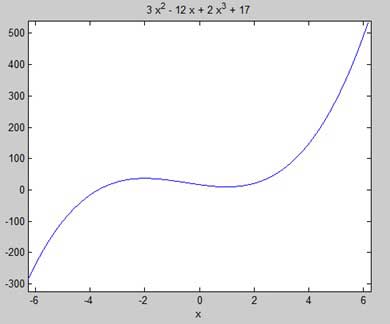
Let us find the stationary points of the function f(x) = 2x3 + 3x2 − 12x + 17
Take the following steps −
First let us enter the function and plot its graph.
syms x
y = 2*x^3 + 3*x^2 - 12*x + 17;   % defining the function
ezplot(y)
MATLAB executes the code and returns the following plot −
Here is Octave equivalent code for the above example −
pkg load symbolic
symbols

x = sym('x');
y = inline("2*x^3 + 3*x^2 - 12*x + 17");

ezplot(y)
print -deps graph.eps
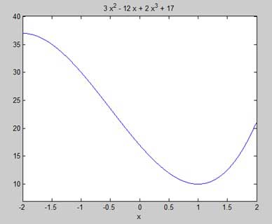
Our aim is to find some local maxima and minima on the graph, so let us find the local maxima and minima for the interval [-2, 2] on the graph.
syms x
y = 2*x^3 + 3*x^2 - 12*x + 17;   % defining the function
ezplot(y, [-2, 2])
MATLAB executes the code and returns the following plot −
Here is Octave equivalent code for the above example −
pkg load symbolic
symbols

x = sym('x');
y = inline("2*x^3 + 3*x^2 - 12*x + 17");

ezplot(y, [-2, 2])
print -deps graph.eps
Next, let us compute the derivative.
g = diff(y)
MATLAB executes the code and returns the following result −
g =
   6*x^2 + 6*x - 12
Here is Octave equivalent of the above calculation −
pkg load symbolic
symbols

x = sym("x");
y = 2*x^3 + 3*x^2 - 12*x + 17;
g = differentiate(y,x)
Octave executes the code and returns the following result −
g =
   -12.0+(6.0)*x+(6.0)*x^(2.0)
Let us solve the derivative function, g, to get the values where it becomes zero.
s = solve(g)
MATLAB executes the code and returns the following result −
s =
   1
   -2
Following is Octave equivalent of the above calculation −
pkg load symbolic
symbols

x = sym("x");
y = 2*x^3 + 3*x^2 - 12*x + 17;
g = differentiate(y,x)
roots([6, 6, -12])
Octave executes the code and returns the following result −
g =

-12.0+(6.0)*x^(2.0)+(6.0)*x
ans =

  -2
   1
This agrees with our plot. So let us evaluate the function f at the critical points x = 1, -2. We can substitute a value in a symbolic function by using the subs command.
subs(y, 1), subs(y, -2)
MATLAB executes the code and returns the following result −
ans =
   10
ans =
   37
Following is Octave equivalent of the above calculation −
pkg load symbolic
symbols

x = sym("x");
y = 2*x^3 + 3*x^2 - 12*x + 17;
g = differentiate(y,x)

roots([6, 6, -12])
subs(y, x, 1), subs(y, x, -2)
ans =
   10.0
ans =
   37.0-4.6734207789940138748E-18*I
Therefore, The minimum and maximum values on the function f(x) = 2x3 + 3x2 − 12x + 17, in the interval [-2,2] are 10 and 37.
Solving Differential Equations
MATLAB provides the dsolve command for solving differential equations symbolically.
The most basic form of the dsolve command for finding the solution to a single equation is
dsolve('eqn')
where eqn is a text string used to enter the equation.
It returns a symbolic solution with a set of arbitrary constants that MATLAB labels C1, C2, and so on.
You can also specify initial and boundary conditions for the problem, as comma-delimited list following the equation as −
dsolve('eqn','cond1', 'cond2',…)
For the purpose of using dsolve command, derivatives are indicated with a D. For example, an equation like f'(t) = -2*f + cost(t) is entered as −
'Df = -2*f + cos(t)'
Higher derivatives are indicated by following D by the order of the derivative.
For example the equation f"(x) + 2f'(x) = 5sin3x should be entered as −
'D2y + 2Dy = 5*sin(3*x)'
Let us take up a simple example of a first order differential equation: y' = 5y.
s = dsolve('Dy = 5*y')
MATLAB executes the code and returns the following result −
s =
   C2*exp(5*t)
Let us take up another example of a second order differential equation as: y" - y = 0, y(0) = -1, y'(0) = 2.
dsolve('D2y - y = 0','y(0) = -1','Dy(0) = 2')
MATLAB executes the code and returns the following result −
ans =
   exp(t)/2 - (3*exp(-t))/2