- Matlab Tutorial
- MATLAB - Home
- MATLAB - Overview
- MATLAB - Environment Setup
- MATLAB - Syntax
- MATLAB - Variables
- MATLAB - Commands
- MATLAB - M-Files
- MATLAB - Data Types
- MATLAB - Operators
- MATLAB - Decisions
- MATLAB - Loops
- MATLAB - Vectors
- MATLAB - Matrix
- MATLAB - Arrays
- MATLAB - Colon Notation
- MATLAB - Numbers
- MATLAB - Strings
- MATLAB - Functions
- MATLAB - Data Import
- MATLAB - Data Output
- MATLAB Advanced
- MATLAB - Plotting
- MATLAB - Graphics
- MATLAB - Algebra
- MATLAB - Calculus
- MATLAB - Differential
- MATLAB - Integration
- MATLAB - Polynomials
- MATLAB - Transforms
- MATLAB - GNU Octave
- MATLAB - Simulink
- MATLAB Useful Resources
- MATLAB - Quick Guide
- MATLAB - Useful Resources
- MATLAB - Discussion
MATLAB - Graphics
This chapter will continue exploring the plotting and graphics capabilities of MATLAB. We will discuss −
- Drawing bar charts
- Drawing contours
- Three dimensional plots
Drawing Bar Charts
The bar command draws a two dimensional bar chart. Let us take up an example to demonstrate the idea.
Example
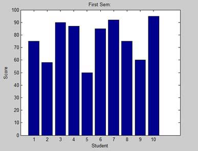
Let us have an imaginary classroom with 10 students. We know the percent of marks obtained by these students are 75, 58, 90, 87, 50, 85, 92, 75, 60 and 95. We will draw the bar chart for this data.
Create a script file and type the following code −
x = [1:10];
y = [75, 58, 90, 87, 50, 85, 92, 75, 60, 95];
bar(x,y), xlabel('Student'),ylabel('Score'),
title('First Sem:')
print -deps graph.eps
When you run the file, MATLAB displays the following bar chart −
Drawing Contours
A contour line of a function of two variables is a curve along which the function has a constant value. Contour lines are used for creating contour maps by joining points of equal elevation above a given level, such as mean sea level.
MATLAB provides a contour function for drawing contour maps.
Example
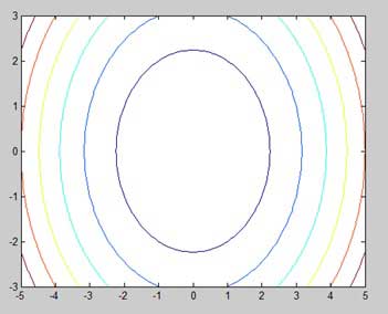
Let us generate a contour map that shows the contour lines for a given function g = f(x, y). This function has two variables. So, we will have to generate two independent variables, i.e., two data sets x and y. This is done by calling the meshgrid command.
The meshgrid command is used for generating a matrix of elements that give the range over x and y along with the specification of increment in each case.
Let us plot our function g = f(x, y), where −5 ≤ x ≤ 5, −3 ≤ y ≤ 3. Let us take an increment of 0.1 for both the values. The variables are set as −
[x,y] = meshgrid(–5:0.1:5, –3:0.1:3);
Lastly, we need to assign the function. Let our function be: x2 + y2
Create a script file and type the following code −
[x,y] = meshgrid(-5:0.1:5,-3:0.1:3);   %independent variables
g = x.^2 + y.^2;                       % our function
contour(x,y,g)                         % call the contour function
print -deps graph.eps
When you run the file, MATLAB displays the following contour map −
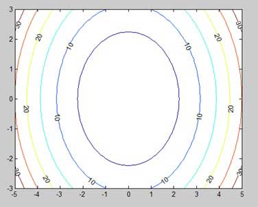
Let us modify the code a little to spruce up the map
[x,y] = meshgrid(-5:0.1:5,-3:0.1:3);   %independent variables
g = x.^2 + y.^2;                       % our function
[C, h] = contour(x,y,g);               % call the contour function
set(h,'ShowText','on','TextStep',get(h,'LevelStep')*2)
print -deps graph.eps
When you run the file, MATLAB displays the following contour map −
Three Dimensional Plots
Three-dimensional plots basically display a surface defined by a function in two variables, g = f (x,y).
As before, to define g, we first create a set of (x,y) points over the domain of the function using the meshgrid command. Next, we assign the function itself. Finally, we use the surf command to create a surface plot.
The following example demonstrates the concept −
Example
Let us create a 3D surface map for the function g = xe-(x2 + y2)
Create a script file and type the following code −
[x,y] = meshgrid(-2:.2:2);
g = x .* exp(-x.^2 - y.^2);
surf(x, y, g)
print -deps graph.eps
When you run the file, MATLAB displays the following 3-D map −
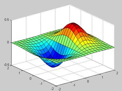
You can also use the mesh command to generate a three-dimensional surface. However, the surf command displays both the connecting lines and the faces of the surface in color, whereas, the mesh command creates a wireframe surface with colored lines connecting the defining points.