- Matlab Tutorial
- MATLAB - Home
- MATLAB - Overview
- MATLAB - Environment Setup
- MATLAB - Syntax
- MATLAB - Variables
- MATLAB - Commands
- MATLAB - M-Files
- MATLAB - Data Types
- MATLAB - Operators
- MATLAB - Decisions
- MATLAB - Loops
- MATLAB - Vectors
- MATLAB - Matrix
- MATLAB - Arrays
- MATLAB - Colon Notation
- MATLAB - Numbers
- MATLAB - Strings
- MATLAB - Functions
- MATLAB - Data Import
- MATLAB - Data Output
- MATLAB Advanced
- MATLAB - Plotting
- MATLAB - Graphics
- MATLAB - Algebra
- MATLAB - Calculus
- MATLAB - Differential
- MATLAB - Integration
- MATLAB - Polynomials
- MATLAB - Transforms
- MATLAB - GNU Octave
- MATLAB - Simulink
- MATLAB Useful Resources
- MATLAB - Quick Guide
- MATLAB - Useful Resources
- MATLAB - Discussion
MATLAB - GNU Octave Tutorial
GNU Octave is a high-level programming language like MATLAB and it is mostly compatible with MATLAB. It is also used for numerical computations.
Octave has the following common features with MATLAB −
- matrices are fundamental data type
- it has built-in support for complex numbers
- it has built-in math functions and libraries
- it supports user-defined functions
GNU Octave is also freely redistributable software. You may redistribute it and/or modify it under the terms of the GNU General Public License (GPL) as published by the Free Software Foundation.
MATLAB vs Octave
Most MATLAB programs run in Octave, but some of the Octave programs may not run in MATLAB because, Octave allows some syntax that MATLAB does not.
For example, MATLAB supports single quotes only, but Octave supports both single and double quotes for defining strings. If you are looking for a tutorial on Octave, then kindly go through this tutorial from beginning which covers both MATLAB as well as Octave.
Compatible Examples
Almost all the examples covered in this tutorial are compatible with MATLAB as well as Octave. Let's try following example in MATLAB and Octave which produces same result without any syntax changes −
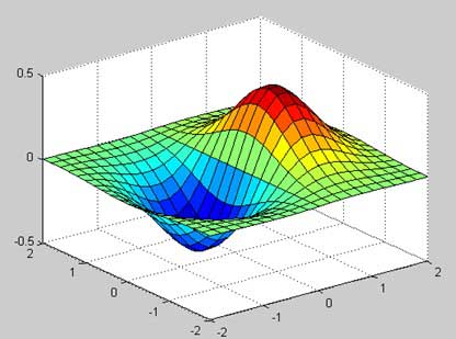
This example creates a 3D surface map for the function g = xe-(x2 + y2). Create a script file and type the following code −
[x,y] = meshgrid(-2:.2:2);
g = x .* exp(-x.^2 - y.^2);
surf(x, y, g)
print -deps graph.eps
When you run the file, MATLAB displays the following 3-D map −
Non-compatible Examples
Though all the core functionality of MATLAB is available in Octave, there are some functionality for example, Differential & Integration Calculus, which does not match exactly in both the languages. This tutorial has tried to give both type of examples where they differed in their syntax.
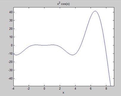
Consider following example where MATLAB and Octave make use of different functions to get the area of a curve: f(x) = x2 cos(x) for −4 ≤ x ≤ 9. Following is MATLAB version of the code −
f = x^2*cos(x);
ezplot(f, [-4,9])
a = int(f, -4, 9)
disp('Area: '), disp(double(a));
When you run the file, MATLAB plots the graph −
The following result is displayed
a =
8*cos(4) + 18*cos(9) + 14*sin(4) + 79*sin(9)

Area:
   0.3326
But to give area of the same curve in Octave, you will have to make use of symbolic package as follows −
pkg load symbolic
symbols

x = sym("x");
f = inline("x^2*cos(x)");

ezplot(f, [-4,9])
print -deps graph.eps

[a, ierror, nfneval] = quad(f, -4, 9);
display('Area: '), disp(double(a));