
Article Categories
- All Categories
-
 Data Structure
-
 Networking
-
 RDBMS
RDBMS
-
 Operating System
-
 Java
Java
-
 MS Excel
-
 iOS
iOS
-
 HTML
HTML
-
 CSS
CSS
-
 Android
-
 Python
-
 C Programming
-
 C++
C++
-
 C#
C#
-
 MongoDB
-
 MySQL
MySQL
-
 Javascript
-
 PHP
PHP
-
 Economics & Finance
Parallel RLC Circuit: Analysis and Example Problems
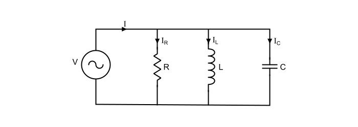
Consider a parallel RLC circuit shown in the figure, where the resistor R, inductor L and capacitor C are connected in parallel and I (RMS) being the total supply current. In a parallel circuit, the voltage V (RMS) across each of the three elements remain same. Hence, for convenience, the voltage may be taken as reference phasor.
Here,
$$\mathrm{\mathit{V}=\mathit{IZ}=\frac{\mathit{I}}{\mathit{Y}}}$$
Where,
- Z= Total impedance of the parallel circuit,
- Y=1/Z= Admittance of the parallel circuit.
The admittance of the parallel circuit is given by,
$$\mathrm{\mathit{Y}=\frac{1}{\mathit{R}}+\frac{1}{\mathit{j\omega L}}+\mathit{j\omega C}=\frac{1}{\mathit{R}}+ {\mathit{j}}(\mathit{\omega C}-\frac{1}{\mathit{\omega L}})=\mathit{G}+\mathit{jB}}$$
Where,
- G=1/R= Conductance of the circuit,
- B=1/X= Susceptance of the circuit,
$$\mathrm{Magnitude\:of\:admittance,|\mathit{Y}|=\sqrt{(\frac{1}{\mathit{R}})^{2}+(\mathit{\omega C}-\frac{1}{\mathit{\omega L}})^{2}}}$$
$$\mathrm{Phase\:angle\:of\:admittance,\:\varphi=\tan^{-1}(\frac{\mathit{\omega C}-\frac{1}{\mathit{\omega L}}}{\frac{1}{\mathit{R}}})=\tan^{-1}(\mathit{R}(\mathit{\omega C}-\frac{1}{\mathit{\omega L}}))}$$
Therefore,
$$\mathrm{\mathit{I}=\mathit{VY}=\mathit{V}×\sqrt{(\frac{1}{\mathit{R}})^{2}+(\mathit{\omega C}-\frac{1}{\mathit{\omega L}})^{2}}\angle\tan^{-1}(\mathit{R}(\mathit{\omega C}-\frac{1}{\mathit{\omega L}}))}$$
Thus,
$$\mathrm{Magnitude\:of\:supply\:current,| \mathit{I}|=\mathit{V}×\sqrt{(\frac{1}{\mathit{R}})^{2}+(\mathit{\omega C}-\frac{1}{\mathit{\omega L}})^{2}}}$$
$$\mathrm{Phase\:angle\:of\:admittance,\:\varphi=\tan^{-1}(\mathit{R}(\mathit{\omega C}-\frac{1}{\mathit{\omega L}}))}$$
Hence, the branch currents are
$$\mathrm{Current\:through\:resistance,\mathit{I}_{\mathit{R}}=\frac{\mathit{V}}{\mathit{R}}=\frac{|\mathit{V}|\angle0^{\circ}}{\mathit{R}}=|\mathit{I}_{\mathit{R}}|\angle0^{\circ}}$$
$$\mathrm{Current\:through\:inductor,\mathit{I}_{L}=\frac{\mathit{V}}{\mathit{X}_{L}}=\frac{|\mathit{V}|\angle0^{\circ}}{\mathit{j\omega L}}=\frac{|\mathit{V}|}{\mathit{\omega L}}\angle(0^{\circ}-90^{\circ})=|\mathit{I}_{L}|\angle(-90^{\circ})}$$
$$\mathrm{Current\:through\:capacitor,\mathit{I}_{c}==\frac{\mathit{V}}{\mathit{X}_{c}}=|\mathit{V}|\angle0^{\circ}(\mathit{j\omega C})=|\mathit{V}| \mathit{\omega C}\angle(+90^{\circ})=|\mathit{I}_{L}|\angle(+90^{\circ})}$$
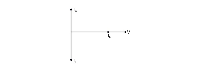
Hence, it is clear that
The current IR through resistance being in phase with the supply voltage.
The current IL through inductor lags the applied voltage by 90°.
The current IC in the capacitor leads the applied voltage by 90°.
The total supply current in the parallel RLC circuit is the phasor sum (bold letters) of above three currents, and not the arithmetic sum i.e.
$$\mathrm{\mathit{I}=\mathit{I}_{\mathit{R}}+\mathit{I}_{\mathit{L}}+\mathit{I}_{\mathit{C}}}$$
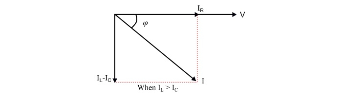
$$\mathrm{Magnitude\:of\:supply,|\mathit{I}|=\sqrt{(\mathit{I}_{\mathit{R}})^2+(\mathit{I}_{\mathit{C}}-\mathit{I}_{\mathit{L}})^2}}$$
The phase angle of supply current I depends upon the magnitude IC and IL.
Three Cases of Parallel RLC Circuit
Case 1 – When,|IL|>|Ic| or XL
Here,
The supply current lags the supply voltage by an angle φ°.
The power factor the circuit is lagging.
The parallel RLC circuit behaves as an inductive circuit.
Case 2 – When,|IL|c| or XL>?XC

Here,
The supply current leads the supply voltage by an angle φ°.
The power factor of the circuit is leading.
The parallel RLC circuit behaves as a capacitive circuit.
Case 3 – When,|IL| = |Ic| or XL = XC

Here,
The supply current being in phase with the supply voltage i.e. angle φ = 0°.
The supply current becomes equal to the current through the resistor, i.e. I = IR.
The power factor of the circuit is unity.
The parallel RLC circuit behaves as a purely resistive circuit.
The parallel RLC circuit in this condition of is called parallel resonating circuit.
Parallel Resonance
The condition of resonance occurs in the parallel RLC circuit, when the susceptance part of admittance is zero. However, admittance is
$$\mathrm{\mathit{Y}=\mathit{G}+\mathit{jB}=\frac{1}{\mathit{R}}+\mathit{j}(\mathit{\omega C}-\frac{1}{\mathit{\omega L}})}$$
At resonance,
$$\mathrm{\mathit{\omega C}-\frac{1}{\mathit{\omega L}}=0}$$
Thus,
$$\mathrm{\mathit{Y}=\frac{1}{\mathit{R}}}$$
The frequency at which resonance occurs is
$$\mathrm{\mathit{\omega_{0} C}-\frac{1}{\mathit{\omega_{0} L}}=0}$$
$$\mathrm{\Rightarrow\:\mathit{\omega_{0}}=\frac{1}{\sqrt{\mathit{LC}}}}$$
The supply current (I) at resonance is
$$\mathrm{\mathit{I}=\mathit{VY}=\frac{\mathit{V}}{\mathit{R}}=\mathit{I}_{\mathit{R}}}$$
$$\mathrm{\Rightarrow\:\mathit{V}=\mathit{IR}=\mathit{I}_{\mathit{R}}\mathit{R}}$$
The magnitude of inductor current (IL) is
$$\mathrm{|\mathit{I}_{L}|=\frac{\mathit{V}}{\mathit{\omega L}}=\frac{\mathit{IR}}{\mathit{\omega L}}=\mathit{IQ}_{0}}$$
$$\mathrm{Where,\mathit{Q}_{0}=\frac{\mathit{R}}{\mathit{\omega L}}=Quality\:factor}$$
The magnitude of capacitor current (IC) at resonance is
$$\mathrm{|\mathit{I}_{c}|=\mathit{V}(\mathit{\omega C})=\mathit{I}(\mathit{\omega R C})=\mathit{IQ}_{0}}$$
Conclusion of Parallel Resonance −
XL=XC or IL = IC, thus the resonant frequency,ω0=$1/\sqrt{LC}$.
Y=1/R i.e.the admittance has minimum value.
Z=R,i.e.the impedance is maximum.
IR=V/R= supply current (I)
| IL |=| IC |=IQ0
The power factor of parallel resonating circuit is unity.
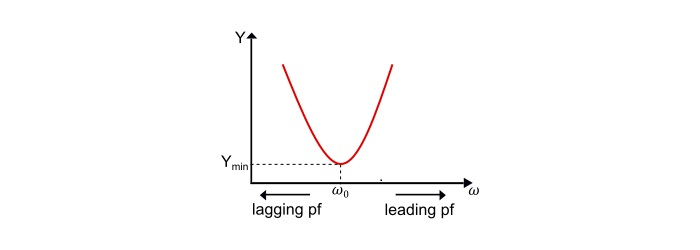
Admittance – Frequency Curve
$$\mathrm{\mathit{Y}=\frac{1}{\mathit{R}}+\mathit{j}(\mathit{\omega C}-\frac{1}{\mathit{\omega L}})}$$
Here,
At the frequencies lower than resonant frequency, XL C or IL > IC , hence the circuit behaves as inductive circuit has lagging power factor.
At the frequencies higher than resonant frequency,XL > XC or IL C hence the circuit behaves as capacitive circuit has leading power factor.
At resonant frequency,XL = XC or IL = IC hence the circuit behaves as purely resistive circuit has unity power factor.
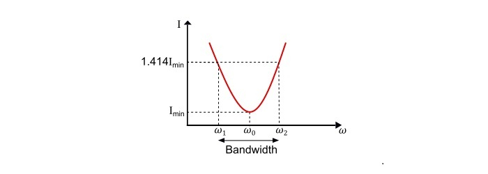
Current – Frequency Curve
$$\mathrm{\mathit{I}=\mathit{VY}\:or\:\mathit{I}\:\alpha\:\mathit{Y}}$$
Thus, current versus frequency curve of the parallel RLC circuit is same as that of admittance versus frequency curve.
Refer the current-frequency curve,
$$\mathrm{Lower\:cut\:off\:frequency,\mathit{\omega}_{1}=-\frac{1}{2\mathit{RC}}+\sqrt{(\frac{1}{2\mathit{RC}})^2+\frac{1}{\mathit{LC}}}}$$
$$\mathrm{Upper\:cut\:off\:frequency,\omega_{2}=+\frac{1}{2\mathit{RC}}+\sqrt{(\frac{1}{2\mathit{RC}})^2+\frac{1}{\mathit{LC}}}}$$
The bandwidth of the circuit is
$$\mathrm{BW=\mathit{\omega}_{2}-\mathit{\omega}_{1}=\frac{1}{\mathit{RC}}=\frac{\mathit{\omega}_{0}}{\mathit{\omega}_{0}\mathit{RC}}=\frac{\mathit{\omega}_{0}}{Q_{0}}}$$
Also,
$$\mathrm{\mathit{\omega}_{1}\:\mathit{\omega}_{2}=\frac{1}{\mathit{LC}}=\mathit{\omega}_{0}^2}$$
$$\mathrm{\Rightarrow\:\mathit{\omega}_{0}=\sqrt{(\mathit{\omega}_{1}\:\mathit{\omega}_{2})}}$$
Hence, the resonant frequency is the geometric mean of half-power frequencies.
Quality Factor of Parallel RLC circuit
$$\mathrm{?\mathit{Q}\:−factor=\frac{Reactive \:Power}{Active\:Power}=\frac{\mathit{R}}{\mathit{\omega L}}=\mathit{\omega RC}}$$
At resonance,
$$\mathrm{\mathit{Q}_{0}-factor=\frac{\mathit{R}}{\omega_{0}\mathit{L}}=\omega_{0}\mathit{RC}}$$
Since, the resonant frequency is
$$\mathrm{\omega_{0}=\frac{1}{\sqrt{\mathit{LC}}}}$$
So, the quality factor of parallel resonant circuit is
$$\mathrm{\mathit{Q}_{0}-factor=\frac{\mathit{R}}{\omega_{0}\mathit{L}}=\mathit{R}\frac{\sqrt{\mathit{LC}}}{\mathit{L}}=\mathit{R}\sqrt{\frac{\mathit{C}}{\mathit{L}}}}$$
Numerical Example
The applied voltage in a parallel RLC circuit is given by
$$\mathrm{\nu=100sin(314t+\frac{\pi}{4})V}$$
If the values of R, L and C be given as 30 Ω, 1.3 mH and 30 μF, Find the total current supplied by the source. Also find the resonant frequency in Hz and corresponding quality factor.
Solution
The RMS value of applied voltage is
$$\mathrm{\mathit{V}=\frac{100\angle45^{\circ}}{\sqrt{2}}=70.72\angle45° V}$$
$$\mathrm{Angular frequency,\omega=314 rad/sec}$$
Here,
$$\mathrm{Admittance,\mathit{Y}=\frac{1}{\mathit{R}}+j(\omega \mathit{C}-\frac{1}{\omega \mathit{L}})}$$
$$\mathrm{?(\omega C-\frac{1}{\omega L})=((314×30×10^{−6})-(\frac{1}{314×1.3×10^{−3}}))=-2.439S}$$
$$\mathrm{∴\mathit{Y}=\frac{1}{30}+j(-2.439)=(0.033−j2.439)}$$
$$\mathrm{|\mathit{Y}|=\sqrt{(0.033)^2+(-2.439)^2}=2.439 S}$$
$$\mathrm{\varphi=\tan^{-1}(-\frac{2.439}{0.033})=-89.22^{\circ}}$$
Thus, the current supplied by the source is
$$\mathrm{\mathit{I}=\mathit{VY}=70.72\angle45°×2.439\angle-89.22°=172.486\angle-44.22°A}$$
The resonant frequency is given by,
$$\mathrm{\mathit{f}_{0}=\frac{1}{2\pi\sqrt(\mathit{LC})}=\frac{1}{2\pi\sqrt{1.3×10^{−3}×30×10^{−6}}}=806.32 Hz}$$
The quality factorcorresponding to resonant frequency is
$$\mathrm{\mathit{Q}_{0}-factor=\mathit{R}\sqrt{\frac{\mathit{C}}{\mathit{L}}}=30×\sqrt{\frac{30×10^{−6}}{1.3×10^{−3}}}=4.557}$$

22K+ Views
