Circuit Analysis with Laplace Transform

Laplace Transform

The Laplace transform is a mathematical tool which is used to convert the differential equation in time domain into the algebraic equations in the frequency domain or s-domain.

Mathematically, if $\mathrm{\mathit{x\left(t\right)}}$ is a time domain function, then its Laplace transform is defined as −

$$\mathrm{\mathit{L\left[\mathit{x}\mathrm{\left(\mathit{t} \right )}\right ]\mathrm{=}X\mathrm{\left( \mathit{s}\right)}\mathrm{=}\int_{-\infty }^{\infty}x\mathrm{\left (\mathit{t} \right )}e^{-st} \:dt}}$$

Circuit Analysis Using Laplace Transform

The Laplace transform can be used to solve the different circuit problems. In order to solve the circuit problems, first the differential equations of the circuits are to be written and then these differential equations are solved by using the Laplace transform. Also, the circuit itself may be converted into s-domain using Laplace transform and then the algebraic equations corresponding to the circuit can be written and solved.

The electrical circuits can have three circuit elements viz. resistor (R), inductor (L) and capacitor (C) and the analysis of these elements using Laplace transform is discussed below.

Pure Resistive Circuit

A circuit consisting of pure resistive element is shown in Figure-1.

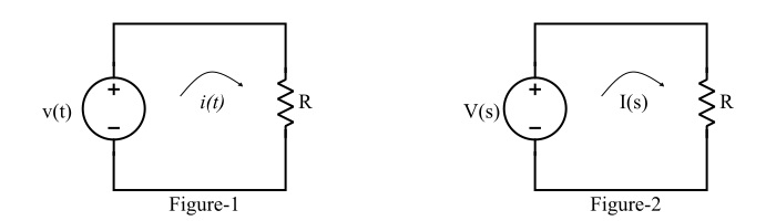
By applying KVL in this circuit, we can write,

$$\mathrm{\mathit{v\mathrm{\left(\mathit{t}\right )}\mathrm{=}Ri\mathrm{\left ( \mathit{t}\right)}}}$$

Therefore, the Laplace transform of this equation is given by,

$$\mathrm{\mathit{V\mathrm{\left(\mathit{s}\right )}\mathrm{=}RI\mathrm{\left ( \mathit{s}\right)}}}$$

Here, it is noted that the resistance R in t-domain remains R in s-domain. The Laplace transformed version of the circuit is shown in Figure-2.

Pure Inductive Circuit

An electrical circuit consisting of pure inductor is shown in Figure-3.

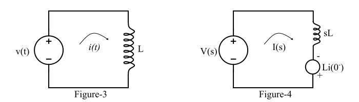
The voltage equation for the pure inductive element is given by,

$$\mathrm{\mathit{v\mathrm{\left(\mathit{t}\right)}\mathrm{=} L\frac{di\mathrm{\left(\mathit{t} \right )}}{dt}}}$$

Taking the Laplace transform of this equation on both sides, we get,

$$\mathrm{\mathit{V\mathrm{\left(\mathit{s}\right)}\mathrm{=} \mathrm{\left[\mathit{sI}\mathrm{\left (\mathit{s} \right)}-\mathit{i\mathrm{\left (0^{-} \right )}}\right]}L}}$$

$$\mathrm{\Rightarrow \mathit{V\mathrm{\left(\mathit{s}\right)}\mathrm{=} sLI\mathrm{\left ( \mathit{s}\right)-\mathit{Li}\mathrm{\left ( 0^{-}\right )}}}}$$

Where,$i\mathrm{\left ( 0^{-}\right )}$ is the initial current flowing through the inductor.

The inductance ($\mathit{L}$) of the element in time domain becomes sL in the s-domain. Also, the circuit current $I\mathrm{\left(\mathit{s}\right)}$ is opposed by the voltage $Li\mathrm{\left(\mathrm{0^{-}}\right)}$. The Laplace transformed version of the pure inductive circuit is shown in Figure-4.

Pure Capacitive Circuit

An electric circuit consisting of pure capacitive element is shown in Figure-5.

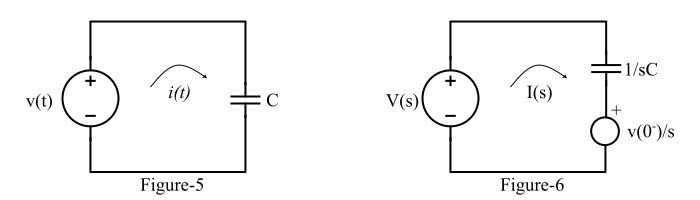
The current flowing through the capacitor is given by,

$$\mathrm{\mathit{i}\mathrm{\left(\mathit{t}\right)}\mathrm{=}\mathit{C\:\frac{dv\left(t\right )}{dt}}}$$

Taking Laplace transform of this equation, we get,

$$\mathrm{\mathit{I}\mathrm{\left(\mathit{s}\right)}\:\mathrm{=}\:\mathit{C}\mathrm{\left[ \mathit{sV\mathrm{\left(s\right)-\mathit{v}\mathrm{\left ( 0^{-} \right )}}}\right ]}\mathrm{=}sCV\mathrm{\left ( s \right )-\mathit{Cv}\mathrm{\left ( 0^{-} \right )}}}$$

$$\mathrm{\therefore \mathit{I}\mathrm{\left(\mathit{s}\right)}\:\mathrm{=}\:sCV\mathrm{\left ( \mathit{s} \right )-\mathit{q}\mathrm{\left ( 0^{-} \right )}}}$$

Also

$$\mathrm{\mathit{V\mathrm{\left ( \mathit{s} \right )}\mathrm{=}\frac{\mathrm{1}}{\mathit{sC}}I\mathrm{\mathit{\left (s\right )}}}+\frac{\mathrm{1}}{\mathit{sC}}\mathit{q}\mathrm{\mathit{\left (\mathrm{0^{-}}\right )}}}$$

$$\mathrm{\therefore \mathit{V\mathrm{\left ( \mathit{s} \right )}\mathrm{=}\frac{I\mathrm{\left (\mathit{s} \right)}}{sC}\mathrm{+}\frac{v\mathrm{\left(\mathrm{0^{-}} \right )}}{s}}}$$

Where, $\mathrm{\mathit{v\mathrm{\left ( 0^{-} \right )}}}$ is the initial voltage across the capacitor.

Here, it is clear that the capacitance (C) in time domain becomes $\mathrm{\left(\frac{1}{\mathit{sc}}\right )}$ in s-domain. Also, the voltage $\mathrm{\left [\frac{\mathit{v}\mathrm{\left ( 0^{-} \right )}}{\mathit{s}} \right ]}$ is introduced in the s-domain which opposes the flow of circuit current. The Laplace transformed version of the pure capacitive circuit is shown in Figure-6.