- OpenCV Python - Home
- OpenCV Python - Overview
- OpenCV Python - Environment
- OpenCV Python - Reading Image
- OpenCV Python - Write Image
- OpenCV Python - Using Matplotlib
- OpenCV Python - Image Properties
- OpenCV Python - Bitwise Operations
- OpenCV Python - Shapes and Text
- OpenCV Python - Mouse Events
- OpenCV Python - Add Trackbar
- OpenCV Python - Resize and Rotate
- OpenCV Python - Image Threshold
- OpenCV Python - Image Filtering
- OpenCV Python - Edge Detection
- OpenCV Python - Histogram
- OpenCV Python - Color Spaces
- OpenCV Python - Transformations
- OpenCV Python - Image Contours
- OpenCV Python - Template Matching
- OpenCV Python - Image Pyramids
- OpenCV Python - Image Addition
- OpenCV Python - Image Blending
- OpenCV Python - Fourier Transform
- OpenCV Python - Capture Videos
- OpenCV Python - Play Videos
- OpenCV Python - Images From Video
- OpenCV Python - Video from Images
- OpenCV Python - Face Detection
- OpenCV Python - Meanshift/Camshift
- OpenCV Python - Feature Detection
- OpenCV Python - Feature Matching
- OpenCV Python - Digit Recognition
- OpenCV Python Resources
- OpenCV Python - Quick Guide
- OpenCV Python - Resources
- OpenCV Python - Discussion
OpenCV-Python - Quick Guide
OpenCV Python - Overview
OpenCV stands for Open Source Computer Vision and is a library of functions which is useful in real time computer vision application programming. The term Computer vision is used for a subject of performing the analysis of digital images and videos using a computer program. Computer vision is an important constituent of modern disciplines such as artificial intelligence and machine learning.
Originally developed by Intel, OpenCV is a cross platform library written in C++ but also has a C Interface Wrappers for OpenCV which have been developed for many other programming languages such as Java and Python. In this tutorial, functionality of OpenCVs Python library will be described.
OpenCV-Python
OpenCV-Python is a Python wrapper around C++ implementation of OpenCV library. It makes use of NumPy library for numerical operations and is a rapid prototyping tool for computer vision problems.
OpenCV-Python is a cross-platform library, available for use on all Operating System (OS) platforms including, Windows, Linux, MacOS and Android. OpenCV also supports the Graphics Processing Unit (GPU) acceleration.
This tutorial is designed for the computer science students and professionals who wish to gain expertise in the field of computer vision applications. Prior knowledge of Python and NumPy library is essential to understand the functionality of OpenCV-Python.
OpenCV Python - Environment Setup
In most of the cases, using pip should be sufficient to install OpenCV-Python on your computer.
The command which is used to install pip is as follows −
pip install opencv-python
Performing this installation in a new virtual environment is recommended. The current version of OpenCV-Python is 4.5.1.48 and it can be verified by following command −
>>> import cv2
>>> cv2.__version__
'4.5.1'
Since OpenCV-Python relies on NumPy, it is also installed automatically. Optionally, you may install Matplotlib for rendering certain graphical output.
On Fedora, you may install OpenCV-Python by the below mentioned command −
$ yum install numpy opencv*
OpenCV-Python can also be installed by building from its source available at http://sourceforge.net Follow the installation instructions given for the same.
OpenCV Python - Reading an image
The CV2 package (name of OpenCV-Python library) provides the imread() function to read an image.
The command to read an image is as follows −
img=cv2.imread(filename, flags)
The flags parameters are the enumeration of following constants −
- cv2.IMREAD_COLOR (1) − Loads a color image.
- cv2.IMREAD_GRAYSCALE (0) − Loads image in grayscale mode
- cv2.IMREAD_UNCHANGED (-1) − Loads image as such including alpha channel
The function will return an image object, which can be rendered using imshow() function. The command for using imshow() function is given below −
cv2.imshow(window-name, image)
The image is displayed in a named window. A new window is created with the AUTOSIZE flag set. The WaitKey() is a keyboard binding function. Its argument is the time in milliseconds.
The function waits for specified milliseconds and keeps the window on display till a key is pressed. Finally, we can destroy all the windows thus created.
The function waits for specified milliseconds and keeps the window on display till a key is pressed. Finally, we can destroy all the windows thus created.
The program to display the OpenCV logo is as follows −
import numpy as np
import cv2
# Load a color image in grayscale
img = cv2.imread('OpenCV_Logo.png',1)
cv2.imshow('image',img)
cv2.waitKey(0)
cv2.destroyAllWindows()
The above program displays the OpenCV logo as follows −
OpenCV Python - Write an image
CV2 package has imwrite() function that saves an image object to a specified file.
The command to save an image with the help of imwrite() function is as follows −
cv2.imwrite(filename, img)
The image format is automatically decided by OpenCV from the file extension. OpenCV supports *.bmp, *.dib , *.jpeg, *.jpg, *.png,*.webp, *.sr,*.tiff, \*.tif etc. image file types.
Example
Following program loads OpenCV logo image and saves its greyscale version when s key is pressed −
import numpy as np
import cv2
# Load an color image in grayscale
img = cv2.imread('OpenCV_Logo.png',0)
cv2.imshow('image',img)
key=cv2.waitKey(0)
if key==ord('s'):
   cv2.imwrite("opencv_logo_GS.png", img)
cv2.destroyAllWindows()
Output
OpenCV Python - Using Matplotlib
Pythons Matplotlib is a powerful plotting library with a huge collection of plotting functions for the variety of plot types. It also has imshow() function to render an image. It gives additional facilities such as zooming, saving etc.
Example
Ensure that Matplotlib is installed in the current working environment before running the following program.
import numpy as np
import cv2
import matplotlib.pyplot as plt
# Load an color image in grayscale
img = cv2.imread('OpenCV_Logo.png',0)
plt.imshow(img)
plt.show()
Output
OpenCV Python - Image Properties
OpenCV reads the image data in a NumPy array. The shape() method of this ndarray object reveals image properties such as dimensions and channels.
The command to use the shape() method is as follows −
>>> img = cv.imread("OpenCV_Logo.png", 1)
>>> img.shape
(222, 180, 3)
In the above command −
- The first two items shape[0] and shape[1] represent width and height of the image.
- Shape[2] stands for a number of channels.
- 3 indicates that the image has Red Green Blue (RGB) channels.
Similarly, the size property returns the size of the image. The command for the size of an image is as follows −
>>> img.size
119880
Each element in the ndarray represents one image pixel.
We can access and manipulate any pixels value, with the help of the command mentioned below.
>>> p=img[50,50]
>>> p
array([ 1, 1, 255], dtype=uint8)
Example
Following code changes the color value of the first 100X100 pixels to black. The imshow() function can verify the result.
>>> for i in range(100):
   for j in range(100):
      img[i,j]=[0,0,0]
Output
The image channels can be split in individual planes by using the split() function. The channels can be merged by using merge() function.
The split() function returns a multi-channel array.
We can use the following command to split the image channels −
>>> img = cv.imread("OpenCV_Logo.png", 1)
>>> b,g,r = cv.split(img)
You can now perform manipulation on each plane.
Suppose we set all pixels in blue channel to 0, the code will be as follows −
>>> img[:, :, 0]=0
>>> cv.imshow("image", img)
The resultant image will be shown as below −
OpenCV Python - Bitwise Operations
Bitwise operations are used in image manipulation and for extracting the essential parts in the image.
Following operators are implemented in OpenCV −
- bitwise_and
- bitwise_or
- bitwise_xor
- bitwise_not
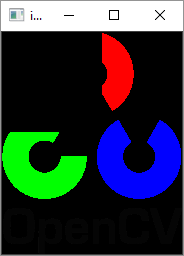
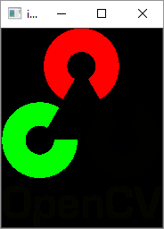
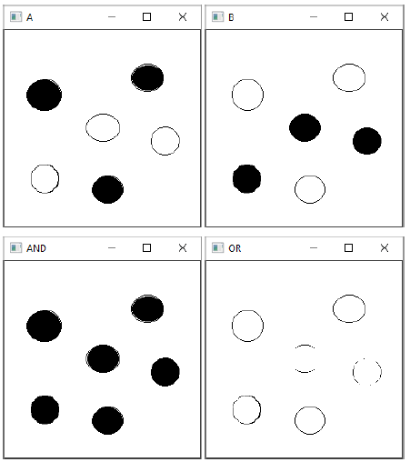
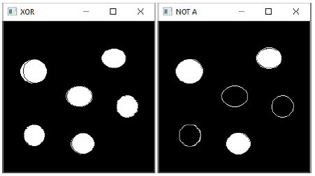
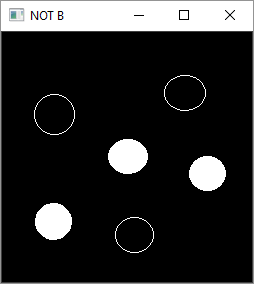
Example 1
To demonstrate the use of these operators, two images with filled and empty circles are taken.
Following program demonstrates the use of bitwise operators in OpenCV-Python −
import cv2
import numpy as np

img1 = cv2.imread('a.png')
img2 = cv2.imread('b.png')

dest1 = cv2.bitwise_and(img2, img1, mask = None)
dest2 = cv2.bitwise_or(img2, img1, mask = None)
dest3 = cv2.bitwise_xor(img1, img2, mask = None)

cv2.imshow('A', img1)
cv2.imshow('B', img2)
cv2.imshow('AND', dest1)
cv2.imshow('OR', dest2)
cv2.imshow('XOR', dest3)
cv2.imshow('NOT A', cv2.bitwise_not(img1))
cv2.imshow('NOT B', cv2.bitwise_not(img2))

if cv2.waitKey(0) & 0xff == 27:
   cv2.destroyAllWindows()
Output
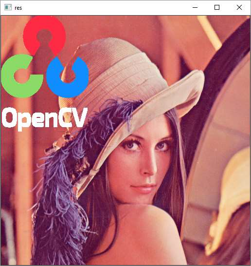
Example 2
In another example involving bitwise operations, the opencv logo is superimposed on another image. Here, we obtain a mask array calling threshold() function on the logo and perform AND operation between them.
Similarly, by NOT operation, we get an inverse mask. Also, we get AND with the background image.
Following is the program which determines the use of bitwise operations −
import cv2 as cv
import numpy as np

img1 = cv.imread('lena.jpg')
img2 = cv.imread('whitelogo.png')
rows,cols,channels = img2.shape
roi = img1[0:rows, 0:cols]
img2gray = cv.cvtColor(img2,cv.COLOR_BGR2GRAY)
ret, mask = cv.threshold(img2gray, 10, 255, cv.THRESH_BINARY)
mask_inv = cv.bitwise_not(mask)
# Now black-out the area of logo
img1_bg = cv.bitwise_and(roi,roi,mask = mask_inv)

# Take only region of logo from logo image.
img2_fg = cv.bitwise_and(img2,img2,mask = mask)
# Put logo in ROI
dst = cv.add(img2_fg, img1_bg)
img1[0:rows, 0:cols ] = dst
cv.imshow(Result,img1)
cv.waitKey(0)
cv.destroyAllWindows()
Output
The masked images give following result −
OpenCV Python - Draw Shapes and Text
In this chapter, we will learn how to draw shapes and text on images with the help of OpenCV-Python. Let us begin by understanding about drawing shapes on images.
Draw Shapes on Images
We need to understand the required functions in OpenCV-Python, which help us to draw the shapes on images.
Functions
The OpenCV-Python package (referred as cv2) contains the following functions to draw the respective shapes.
| Function | Description | Command |
|---|---|---|
| cv2.line() | Draws a line segment connecting two points. | cv2.line(img, pt1, pt2, color, thickness) |
| cv2.circle() | Draws a circle of given radius at given point as center | cv2.circle(img, center, radius, color, thickness) |
| cv2.rectangle | Draws a rectangle with given points as top-left and bottom-right. | cv2.rectangle(img, pt1, pt2, color, thickness) |
| cv2.ellipse() | Draws a simple or thick elliptic arc or fills an ellipse sector. | cv2.ellipse(img, center, axes, angle, startAngle, endAngle, color, thickness) |
Parameters
The common parameters to the above functions are as follows −
| Sr.No. | Function & Description |
|---|---|
| 1 | img The image where you want to draw the shapes |
| 2 | color Color of the shape. for BGR, pass it as a tuple. For grayscale, just pass the scalar value. |
| 3 | thickness Thickness of the line or circle etc. If -1 is passed for closed figures like circles, it will fill the shape. |
| 4 | lineType Type of line, whether 8-connected, anti-aliased line etc. |
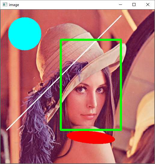
Example
Following example shows how the shapes are drawn on top of an image. The program for the same is given below −
import numpy as np
import cv2
img = cv2.imread('LENA.JPG',1)
cv2.line(img,(20,400),(400,20),(255,255,255),3)
cv2.rectangle(img,(200,100),(400,400),(0,255,0),5)
cv2.circle(img,(80,80), 55, (255,255,0), -1)
cv2.ellipse(img, (300,425), (80, 20), 5, 0, 360, (0,0,255), -1)
cv2.imshow('image',img)
cv2.waitKey(0)
cv2.destroyAllWindows()
Output
Draw Text
The cv2.putText() function is provided to write a text on the image. The command for the same is as follows −
img, text, org, fontFace, fontScale, color, thickness)
Fonts
OpenCV supports the following fonts −
| Font Name | Font Size |
|---|---|
| FONT_HERSHEY_SIMPLEX | 0 |
| FONT_HERSHEY_PLAIN | 1 |
| FONT_HERSHEY_DUPLEX | 2 |
| FONT_HERSHEY_COMPLEX | 3 |
| FONT_HERSHEY_TRIPLEX | 4 |
| FONT_HERSHEY_COMPLEX_SMALL | 5 |
| FONT_HERSHEY_SCRIPT_SIMPLEX | 6 |
| FONT_HERSHEY_SCRIPT_COMPLEX | 7 |
| FONT_ITALIC | 16 |
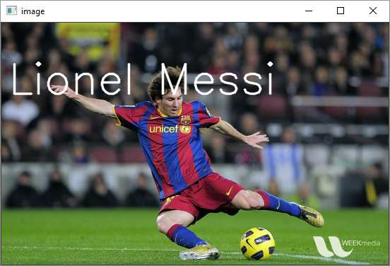
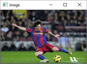
Example
Following program adds a text caption to a photograph showing Lionel Messi, the famous footballer.
import numpy as np
import cv2
img = cv2.imread('messi.JPG',1)
txt="Lionel Messi"
font = cv2.FONT_HERSHEY_SIMPLEX
cv2.putText(img,txt,(10,100), font, 2,(255,255,255),2,cv2.LINE_AA)

cv2.imshow('image',img)
cv2.waitKey(0)
cv2.destroyAllWindows()
Output
OpenCV Python - Handling Mouse Events
OpenCV is capable of registering various mouse related events with a callback function. This is done to initiate a certain user defined action depending on the type of mouse event.
| Sr.No | Mouse event & Description |
|---|---|
| 1 | cv.EVENT_MOUSEMOVE When the mouse pointer has moved over the window. |
| 2 | cv.EVENT_LBUTTONDOWN Indicates that the left mouse button is pressed. |
| 3 | cv.EVENT_RBUTTONDOWN Event of that the right mouse button is pressed. |
| 4 | cv.EVENT_MBUTTONDOWN Indicates that the middle mouse button is pressed. |
| 5 | cv.EVENT_LBUTTONUP When the left mouse button is released. |
| 6 | cv.EVENT_RBUTTONUP When the right mouse button is released. |
| 7 | cv.EVENT_MBUTTONUP Indicates that the middle mouse button is released. |
| 8 | cv.EVENT_LBUTTONDBLCLK This event occurs when the left mouse button is double clicked. |
| 9 | cv.EVENT_RBUTTONDBLCLK Indicates that the right mouse button is double clicked. |
| 10 | cv.EVENT_MBUTTONDBLCLK Indicates that the middle mouse button is double clicked. |
| 11 | cv.EVENT_MOUSEWHEEL Positive for forward and negative for backward scrolling. |
To fire a function on a mouse event, it has to be registered with the help of setMouseCallback() function. The command for the same is as follows −
cv2.setMouseCallback(window, callbak_function)
This function passes the type and location of the event to the callback function for further processing.
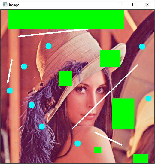
Example 1
Following code draws a circle whenever left button double click event occurs on the window showing an image as background −
import numpy as np
import cv2 as cv
# mouse callback function
def drawfunction(event,x,y,flags,param):
   if event == cv.EVENT_LBUTTONDBLCLK:
      cv.circle(img,(x,y),20,(255,255,255),-1)
img = cv.imread('lena.jpg')
cv.namedWindow('image')
cv.setMouseCallback('image',drawfunction)
while(1):
   cv.imshow('image',img)
   key=cv.waitKey(1)
   if key == 27:
      break
cv.destroyAllWindows()
Output
Run the above program and double click at random locations. The similar output will appear −
Example 2
Following program interactively draws either rectangle, line or circle depending on user input (1,2 or 3) −
import numpy as np
import cv2 as cv
# mouse callback function
drawing=True
shape='r'
def draw_circle(event,x,y,flags,param):
global x1,x2
if event == cv.EVENT_LBUTTONDOWN:
drawing = True
x1,x2 = x,y
elif event == cv.EVENT_LBUTTONUP:
drawing = False
if shape == 'r':
cv.rectangle(img,(x1,x2),(x,y),(0,255,0),-1)
if shape == 'l':
cv.line(img,(x1,x2),(x,y),(255,255,255),3)
if shape=='c':
cv.circle(img,(x,y), 10, (255,255,0), -1)
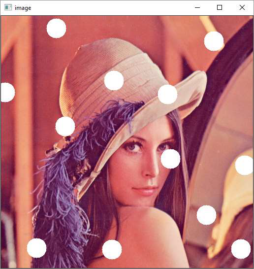
img = cv.imread('lena.jpg')
cv.namedWindow('image')
cv.setMouseCallback('image',draw_circle)
while(1):
cv.imshow('image',img)
key=cv.waitKey(1)
if key==ord('1'):
shape='r'
if key==ord('2'):
shape='l'
if key==ord('3'):
shape='c'
#print (shape)
if key == 27:
break
cv.destroyAllWindows()
On the window surface, a rectangle is drawn between the coordinates of the mouse left button down and up if 1 is pressed.
If user choice is 2, a line is drawn using coordinates as endpoints.
On choosing 3 for the circle, it is drawn at the coordinates of the mouse up event.
Following image will be the output after the successful execution of the above mentioned program −
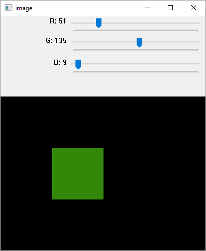
OpenCV Python - Add Trackbar
Trackbar in OpenCV is a slider control which helps in picking a value for the variable from a continuous range by manually sliding the tab over the bar. Position of the tab is synchronised with a value.
The createTrackbar() function creates a Trackbar object with the following command −
cv2.createTrackbar(trackbarname, winname, value, count, TrackbarCallback)
In the following example, three trackbars are provided for the user to set values of R, G and B from the grayscale range 0 to 255.
Using the track bar position values, a rectangle is drawn with the fill colour corresponding to RGB colour value.
Example
Following program is for adding a trackbar −
import numpy as np
import cv2 as cv
img = np.zeros((300,400,3), np.uint8)
cv.namedWindow('image')
def nothing(x):
   pass

# create trackbars for color change
cv.createTrackbar('R','image',0,255,nothing)
cv.createTrackbar('G','image',0,255,nothing)
cv.createTrackbar('B','image',0,255,nothing)

while(1):
   cv.imshow('image',img)
   k = cv.waitKey(1) & 0xFF
   if k == 27:
      break
   # get current positions of four trackbars
   r = cv.getTrackbarPos('R','image')
   g = cv.getTrackbarPos('G','image')
   b = cv.getTrackbarPos('B','image')

   #s = cv.getTrackbarPos(switch,'image')
   #img[:] = [b,g,r]
   cv.rectangle(img, (100,100),(200,200), (b,g,r),-1)
   cv.destroyAllWindows()
Output
OpenCV Python - Resize and Rotate an Image
In this chapter, we will learn how to resize and rotate an image with the help of OpenCVPython.
Resize an Image
It is possible to scale up or down an image with the use of cv2.resize() function.
The resize() function is used as follows −
resize(src, dsize, dst, fx, fy, interpolation)
In general, interpolation is a process of estimating values between known data points.
When graphical data contains a gap, but data is available on either side of the gap or at a few specific points within the gap. Interpolation allows us to estimate the values within the gap.
In the above resize() function, interpolation flags determine the type of interpolation used for calculating size of destination image.
Types of Interpolation
The types of interpolation are as follows −
INTER_NEAREST − A nearest-neighbor interpolation.
INTER_LINEAR − A bilinear interpolation (used by default)
INTER_AREA − Resampling using pixel area relation. It is a preferred method for image decimation but when the image is zoomed, it is similar to the INTER_NEAREST method.
INTER_CUBIC − A bicubic interpolation over 4x4 pixel neighborhood
INTER_LANCZOS4 − A Lanczos interpolation over 8x8 pixel neighborhood
Preferable interpolation methods are cv2.INTER_AREA for shrinking and cv2.INTER_CUBIC (slow) & cv2.INTER_LINEAR for zooming.
Example
Following code resizes the messi.jpg image to half its original height and width.
import numpy as np
import cv2
img = cv2.imread('messi.JPG',1)
height, width = img.shape[:2]
res = cv2.resize(img,(int(width/2), int(height/2)), interpolation =
cv2.INTER_AREA)

cv2.imshow('image',res)
cv2.waitKey(0)
cv2.destroyAllWindows()
Output
Rotate an image
OpenCV uses affine transformation functions for operations on images such as translation and rotation. The affine transformation is a transformation that can be expressed in the form of a matrix multiplication (linear transformation) followed by a vector addition (translation).
The cv2 module provides two functions cv2.warpAffine and cv2.warpPerspective, with which you can have all kinds of transformations. cv2.warpAffine takes a 2x3 transformation matrix while cv2.warpPerspective takes a 3x3 transformation matrix as input.
To find this transformation matrix for rotation, OpenCV provides a function, cv2.getRotationMatrix2D, which is as follows −
getRotationMatrix2D(center, angle, scale)
We then apply the warpAffine function to the matrix returned by getRotationMatrix2D() function to obtain rotated image.
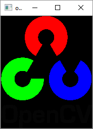
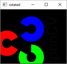
Following program rotates the original image by 90 degrees without changing the dimensions −
Example
import numpy as np
import cv2
img = cv2.imread('OpenCV_Logo.png',1)
h, w = img.shape[:2]

center = (w / 2, h / 2)
mat = cv2.getRotationMatrix2D(center, 90, 1)
rotimg = cv2.warpAffine(img, mat, (h, w))
cv2.imshow('original',img)
cv2.imshow('rotated', rotimg)
cv2.waitKey(0)
cv2.destroyAllWindows()
Output
Original Image
Rotated Image
OpenCV Python - Image Threshold
In digital image processing, the thresholding is a process of creating a binary image based on a threshold value of pixel intensity. Thresholding process separates the foreground pixels from background pixels.
OpenCV provides functions to perform simple, adaptive and Otsus thresholding.
In simple thresholding, all pixels with value less than threshold are set to zero, rest to the maximum pixel value. This is the simplest form of thresholding.
The cv2.threshold() function has the following definition.
cv2.threshold((src, thresh, maxval, type, dst)
Parameters
The parameters for the image thresholding are as follows −
- Src: Input array.
- Dst: Output array of same size.
- Thresh: Threshold value.
- Maxval: Maximum value.
- Type: Thresholding type.
Types of Thresholding
Other types of thresholding are enumerated as below −
| Sr.No | Type & Function |
|---|---|
| 1 | cv.THRESH_BINARY dst(x,y) = maxval if src(x,y)>thresh 0 otherwise |
| 2 | cv.THRESH_BINARY_INV dst(x,y)=0 if src(x,y)>thresh maxval otherwise |
| 3 | cv.THRESH_TRUNC dst(x,y)=threshold if src(x,y)>thresh src(x,y) otherwise |
| 4 | cv.THRESH_TOZERO dst(x,y)=src(x,y) if src(x,y)>thresh 0 otherwise |
| 5 | cv.THRESH_TOZERO_INV dst(x,y)=0 if src(x,y)>thresh src(x,y)otherwise |
These threshold types result in operation on input image according to following diagram −
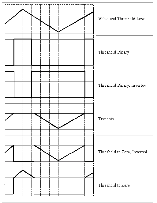
The threshold() function returns threshold used and threshold image.
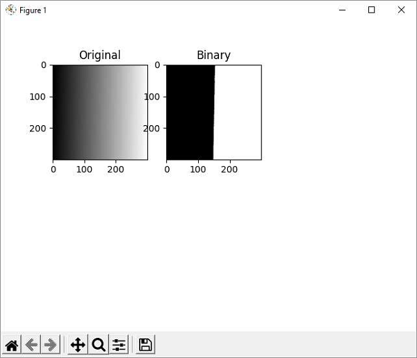
Following program produces a binary image from the original with a gradient of grey values from 255 to 0 by setting a threshold to 127.
Example
Original and resultant threshold binary images are plotted side by side using Matplotlib library.
import cv2 as cv
import numpy as np
from matplotlib import pyplot as plt
img = cv.imread('gradient.png',0)
ret,img1 = cv.threshold(img,127,255,cv.THRESH_BINARY)

plt.subplot(2,3,1),plt.imshow(img,'gray',vmin=0,vmax=255)
plt.title('Original')
plt.subplot(2,3,2),plt.imshow(img1,'gray',vmin=0,vmax=255)
plt.title('Binary')
plt.show()
Output
The adaptive thresholding determines the threshold for a pixel based on a small region around it. So, different thresholds for different regions of the same image are obtained. This gives better results for images with varying illumination.
The cv2.adaptiveThreshold() method takes following input arguments −
cv.adaptiveThreshold( src, maxValue, adaptiveMethod, thresholdType, blockSize, C[, dst] )
The adaptiveMethod has following enumerated values −
cv.ADAPTIVE_THRESH_MEAN_C − The threshold value is the mean of the neighbourhood area minus the constant C.
cv.ADAPTIVE_THRESH_GAUSSIAN_C − The threshold value is a Gaussianweighted sum of the neighbourhood values minus the constant C.
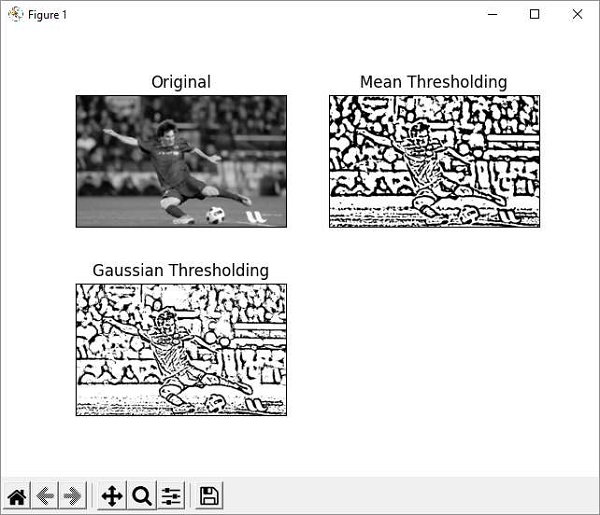
Example
In the example below, the original image (messi.jpg is applied with mean and Gaussian adaptive thresholding.
import cv2 as cv
import numpy as np
from matplotlib import pyplot as plt
img = cv.imread('messi.jpg',0)
img = cv.medianBlur(img,5)
th1 = cv.adaptiveThreshold(img,255,cv.ADAPTIVE_THRESH_MEAN_C,\
   cv.THRESH_BINARY,11,2)
th2 = cv.adaptiveThreshold(img,255,cv.ADAPTIVE_THRESH_GAUSSIAN_C,\
   cv.THRESH_BINARY,11,2)
titles = ['Original', 'Mean Thresholding', 'Gaussian Thresholding']
images = [img, th1, th2]
for i in range(3):
   plt.subplot(2,2,i+1),plt.imshow(images[i],'gray')
   plt.title(titles[i])
   plt.xticks([]),plt.yticks([])
plt.show()
Output
Original as well as adaptive threshold binary images are plotted by using matplotlib as shown below −
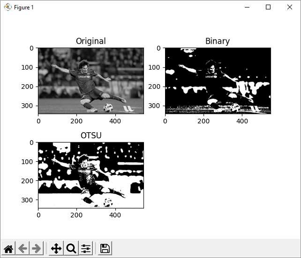
Example
OTSU algorithm determines the threshold value automatically from the image histogram. We need to pass the cv.THRES_OTSU flag in addition to the THRESH-BINARY flag.
import cv2 as cv
import numpy as np
from matplotlib import pyplot as plt
img = cv.imread('messi.jpg',0)
# global thresholding
ret1,img1 = cv.threshold(img,127,255,cv.THRESH_BINARY)
# Otsu's thresholding
ret2,img2 = cv.threshold(img,0,255,cv.THRESH_BINARY+cv.THRESH_OTSU)
plt.subplot(2,2,1),plt.imshow(img,'gray',vmin=0,vmax=255)
plt.title('Original')
plt.subplot(2,2,2),plt.imshow(img1,'gray')

plt.title('Binary')
plt.subplot(2,2,3),plt.imshow(img2,'gray')
plt.title('OTSU')
plt.show()
Output
The matplotlibs plot result is as follows −
OpenCV Python - Image Filtering
An image is basically a matrix of pixels represented by binary values between 0 to 255 corresponding to gray values. A color image will be a three dimensional matrix with a number of channels corresponding to RGB.
Image filtering is a process of averaging the pixel values so as to alter the shade, brightness, contrast etc. of the original image.
By applying a low pass filter, we can remove any noise in the image. High pass filters help in detecting the edges.
The OpenCV library provides cv2.filter2D() function. It performs convolution of the original image by a kernel of a square matrix of size 3X3 or 5X5 etc.
Convolution slides a kernel matrix across the image matrix horizontally and vertically. For each placement, add all pixels under the kernel, take the average of pixels under the kernel and replace the central pixel with the average value.
Perform this operation for all pixels to obtain the output image pixel matrix. Refer the diagram given below −
The cv2.filter2D() function requires input array, kernel matrix and output array parameters.
Example
Following figure uses this function to obtain an averaged image as a result of 2D convolution. The program for the same is as follows −
import numpy as np
import cv2 as cv
from matplotlib import pyplot as plt
img = cv.imread('opencv_logo_gs.png')
kernel = np.ones((3,3),np.float32)/9
dst = cv.filter2D(img,-1,kernel)
plt.subplot(121),plt.imshow(img),plt.title('Original')
plt.xticks([]), plt.yticks([])
plt.subplot(122),plt.imshow(dst),plt.title('Convolved')
plt.xticks([]), plt.yticks([])
plt.show()
Output
Types of Filtering Function
Other types of filtering function in OpenCV includes −
BilateralFilter − Reduces unwanted noise keeping edges intact.
BoxFilter − This is an average blurring operation.
GaussianBlur − Eliminates high frequency content such as noise and edges.
MedianBlur − Instead of average, it takes the median of all pixels under the kernel and replaces the central value.
OpenCV Python - Edge Detection
An edge here means the boundary of an object in the image. OpenCV has a cv2.Canny() function that identifies the edges of various objects in an image by implementing Cannys algorithm.
Canny edge detection algorithm was developed by John Canny. According to it, objects edges are determined by performing following steps −
First step is to reduce the noisy pixels in the image. This is done by applying 5X5 Gaussian Filter.
Second step involves finding the intensity gradient of the image. The smooth image of the first stage is filtered by applying the Sobel operator to obtain first order derivatives in horizontal and vertical directions (Gx and Gy).
The root mean square value gives edge gradient and tan inverse ratio of derivatives gives the direction of edge.
$$\mathrm{Edge \:gradient\:G\:=\:\sqrt{G_x^2+G_y^2}}$$
$$\mathrm{Angle\:\theta\:=\:\tan^{-1}(\frac{G_{y}}{G_{x}})}$$
After getting gradient magnitude and direction, a full scan of the image is done to remove any unwanted pixels which may not constitute the edge.
Next step is to perform hysteresis thresholding by using minval and maxval thresholds. Intensity gradients less than minval and maxval are non-edges so discarded. Those in between are treated as edge points or non-edges based on their connectivity.
All these steps are performed by OpenCVs cv2.Canny() function which needs the input image array and minval and maxval parameters.
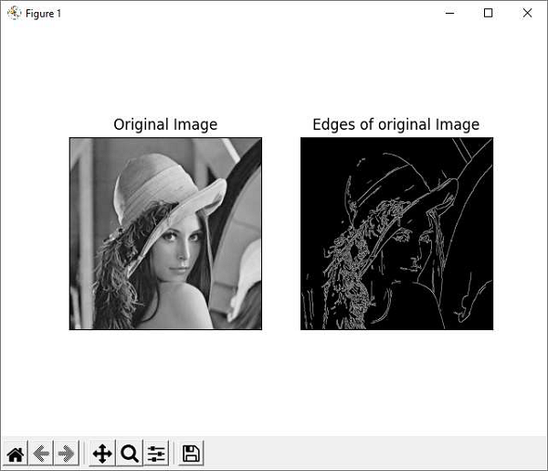
Example
Heres the example of canny edge detection. The program for the same is as follows −
import numpy as np
import cv2 as cv
from matplotlib import pyplot as plt
img = cv.imread('lena.jpg', 0)
edges = cv.Canny(img,100,200)
plt.subplot(121),plt.imshow(img,cmap = 'gray')
plt.title('Original Image'), plt.xticks([]), plt.yticks([])
plt.subplot(122),plt.imshow(edges,cmap = 'gray')
plt.title('Edges of original Image'), plt.xticks([]), plt.yticks([])
plt.show()
Output
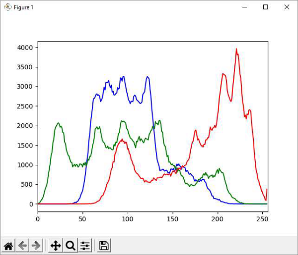
OpenCV Python - Histogram
Histogram shows the intensity distribution in an image. It plots the pixel values (0 to 255) on X axis and number of pixels on Y axis.
By using histogram, one can understand the contrast, brightness and intensity distribution of the specified image. The bins in a histogram represent incremental parts of the values on X axis.
In our case, it is the pixel value and the default bin size is one.
In OpenCV library, the function cv2.calcHist() function which computes the histogram from the input image. The command for the function is as follows −
cv.calcHist(images, channels, mask, histSize, ranges)
Parameters
The cv2.calcHist() functions parameters are as follows −
images − It is the source image of type uint8 or float32, in square brackets, i.e., "[img]".
channels − It is the index of the channel for which we calculate histogram. For a grayscale image, its value is [0]. For BGR images, you can pass [0], [1] or [2] to calculate the histogram of each channel.
mask − Mask image is given as "None" for full image. For a particular region of image, you have to create a mask image for that and give it as a mask.
histSize − This represents our BIN count.
ranges − Normally, it is [0,256].
Histogram using Matplotlib
A histogram plot can be obtained either with the help of Matplotlibs pyplot.plot() function or by calling Polylines() function from OpenCV library.
Example
Following program computes histogram for each channel in the image (lena.jpg) and plots the intensity distribution for each channel −
import numpy as np
import cv2 as cv
from matplotlib import pyplot as plt
img = cv.imread('lena.jpg')
color = ('b','g','r')
for i,col in enumerate(color):
   hist = cv.calcHist([img],[i],None,[256],[0,256])
   plt.plot(hist, color = col)
   plt.xlim([0,256])
plt.show()
Output
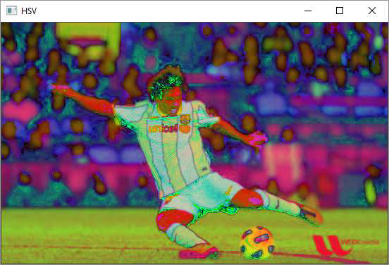
OpenCV Python - Color Spaces
A color space is a mathematical model describing how colours can be represented. It is described in a specific, measurable, and fixed range of possible colors and luminance values.
OpenCV supports following well known color spaces −
RGB Color space − It is an additive color space. A color value is obtained by combination of red, green and blue colour values. Each is represented by a number ranging between 0 to 255.
HSV color space − H, S and V stand for Hue, Saturation and Value. This is an alternative color model to RGB. This model is supposed to be closer to the way a human eye perceives any colour. Hue value is between 0 to 179, whereas S and V numbers are between 0 to 255.
CMYK color space − In contrast to RGB, CMYK is a subtractive color model. The alphabets stand for Cyan, Magenta, Yellow and Black. White light minus red leaves cyan, green subtracted from white leaves magenta, and white minus blue returns yellow. All the values are represented on the scale of 0 to 100 %.
CIELAB color space − The LAB color space has three components which are L for lightness, A color components ranging from Green to Magenta and B for components from Blue to Yellow.
YCrCb color space − Here, Cr stands for R-Y and Cb stands for B-Y. This helps in separation of luminance from chrominance into different channels.
OpenCV supports conversion of image between color spaces with the help of cv2.cvtColor() function.
The command for the cv2.cvtColor() function is as follows −
cv.cvtColor(src, code, dst)
Conversion Codes
The conversion is governed by following predefined conversion codes.
| Sr.No. | Conversion Code & Function |
|---|---|
| 1 | cv.COLOR_BGR2BGRA Add alpha channel to RGB or BGR image. |
| 2 | cv.COLOR_BGRA2BGR Remove alpha channel from RGB or BGR image. |
| 3 | cv.COLOR_BGR2GRAY Convert between RGB/BGR and grayscale. |
| 4 | cv.COLOR_BGR2YCrCb Convert RGB/BGR to luma-chroma |
| 5 | cv.COLOR_BGR2HSV Convert RGB/BGR to HSV |
| 6 | cv.COLOR_BGR2Lab Convert RGB/BGR to CIE Lab |
| 7 | cv.COLOR_HSV2BGR Backward conversions HSV to RGB/BGR |
Example
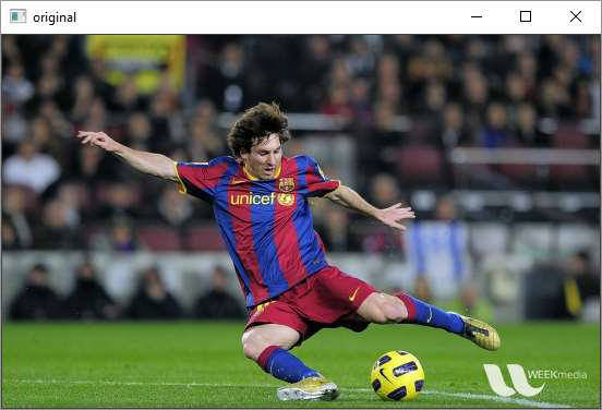
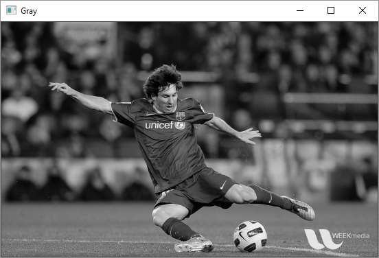
Following program shows the conversion of original image with RGB color space to HSV and Gray schemes −
import cv2
img = cv2.imread('messi.jpg')
img1 = cv2.cvtColor(img, cv2.COLOR_BGR2GRAY )
img2 = cv2.cvtColor(img, cv2.COLOR_BGR2HSV)
# Displaying the image
cv2.imshow('original', img)
cv2.imshow('Gray', img1)
cv2.imshow('HSV', img2)
Output
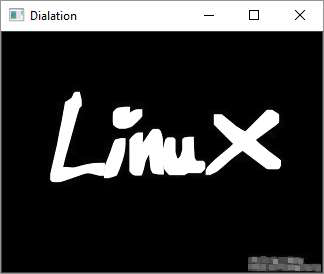
OpenCV Python - Morphological Transformations
Simple operations on an image based on its shape are termed as morphological transformations. The two most common transformations are erosion and dilation.
Erosion
Erosion gets rid of the boundaries of the foreground object. Similar to 2D convolution, a kernel is slide across the image A. The pixel in the original image is retained, if all the pixels under the kernel are 1.
Otherwise it is made 0 and thus, it causes erosion. All the pixels near the boundary are discarded. This process is useful for removing white noises.
The command for the erode() function in OpenCV is as follows −
cv.erode(src, kernel, dst, anchor, iterations)
Parameters
The erode() function in OpenCV uses following parameters −
The src and dst parameters are input and output image arrays of the same size. Kernel is a matrix of structuring elements used for erosion. For example, 3X3 or 5X5.
The anchor parameter is -1 by default which means the anchor element is at center. Iterations refers to the number of times erosion is applied.
Dilation
It is just the opposite of erosion. Here, a pixel element is 1, if at least one pixel under the kernel is 1. As a result, it increases the white region in the image.
The command for the dilate() function is as follows −
cv.dilate(src, kernel, dst, anchor, iterations)
Parameters
The dilate() function has the same parameters such as that of erode() function. Both functions can have additional optional parameters as BorderType and borderValue.
BorderType is an enumerated type of image boundaries (CONSTANT, REPLICATE, TRANSPERANT etc.)
borderValue is used in case of a constant border. By default, it is 0.
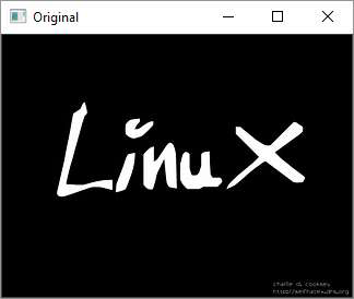
Example
Given below is an example program showing erode() and dilate() functions in use −
import cv2 as cv
import numpy as np
img = cv.imread('LinuxLogo.jpg',0)
kernel = np.ones((5,5),np.uint8)
erosion = cv.erode(img,kernel,iterations = 1)
dilation = cv.dilate(img,kernel,iterations = 1)
cv.imshow('Original', img)
cv.imshow('Erosion', erosion)
cv.imshow('Dialation', dilation)
Output
Original Image
Erosion
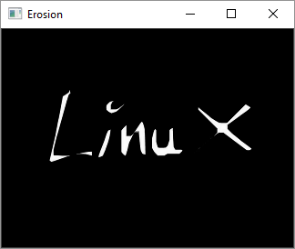
Dilation
OpenCV Python - Image Contours
Contour is a curve joining all the continuous points along the boundary having the same color or intensity. The contours are very useful for shape analysis and object detection.
Find Contour
Before finding contours, we should apply threshold or canny edge detection. Then, by using findContours() method, we can find the contours in the binary image.
The command for the usage of findContours()function is as follows −
cv.findContours(image, mode, method, contours)
Parameters
The parameters of the findContours() function are as follows −
- image − Source, an 8-bit single-channel image.
- mode − Contour retrieval mode.
- method − Contour approximation method.
The mode parameters values are enumerated as follows −
cv.RETR_EXTERNAL − Retrieves only the extreme outer contours.
cv.RETR_LIST − Retrieves all of the contours without establishing any hierarchical relationships.
cv.RETR_CCOMP − Retrieves all of the contours and organizes them into a twolevel hierarchy.
cv.RETR_TREE − Retrieves all of the contours and reconstructs a full hierarchy of nested contours.
On the other hand, approximation method can be one from the following −
cv.CHAIN_APPROX_NONE − Stores absolutely all the contour points.
cv.CHAIN_APPROX_SIMPLE − Compresses horizontal, vertical, and diagonal segments and leaves only their end points.
Draw Contour
After detecting the contour vectors, contours are drawn over the original image by using the cv.drawContours() function.
The command for the cv.drawContours() function is as follows −
cv.drawContours(image, contours, contourIdx, color)
Parameters
The parameters of the drawContours() function are as follows −
- image − Destination image.
- contours − All the input contours. Each contour is stored as a point vector.
- contourIdx − Parameter indicating a contour to draw. If it is negative, all the contours are drawn.
- color − Color of the contours.
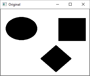
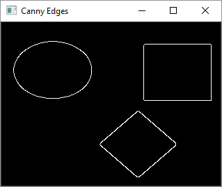
Example
Following code is an example of drawing contours on an input image having three shapes filled with black colours.
In the first step, we obtain a gray image and then perform the canny edge detection.
On the resultant image, we then call findContours() function. Its result is a point vector. We then call the drawContours() function.
The complete code is as below −
import cv2
import numpy as np

img = cv2.imread('shapes.png')
cv2.imshow('Original', img)
gray = cv2.cvtColor(img, cv2.COLOR_BGR2GRAY)

canny = cv2.Canny(gray, 30, 200)

contours, hierarchy = cv2.findContours(canny,
   cv2.RETR_EXTERNAL, cv2.CHAIN_APPROX_NONE)
print("Number of Contours = " ,len(contours))
cv2.imshow('Canny Edges', canny)

cv2.drawContours(img, contours, -1, (0, 255, 0), 3)

cv2.imshow('Contours', img)
cv2.waitKey(0)
cv2.destroyAllWindows()
Output
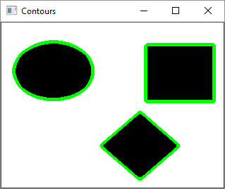
The original image, after canny edge detection and one with contours drawn will be displayed in separate windows as shown here −
After the canny edge detection, the image will be as follows −
After the contours are drawn, the image will be as follows −
OpenCV Python - Template Matching
The technique of template matching is used to detect one or more areas in an image that matches with a sample or template image.
Cv.matchTemplate() function in OpenCV is defined for the purpose and the command for the same is as follows:
cv.matchTemplate(image, templ, method)
Where image is the input image in which the templ (template) pattern is to be located. The method parameter takes one of the following values −
- cv.TM_CCOEFF,
- cv.TM_CCOEFF_NORMED, cv.TM_CCORR,
- cv.TM_CCORR_NORMED,
- cv.TM_SQDIFF,
- cv.TM_SQDIFF_NORMED
This method slides the template image over the input image. This is a similar process to convolution and compares the template and patch of input image under the template image.
It returns a grayscale image, whose each pixel denotes how much it matches with the template. If the input image is of size (WxH) and template image is of size (wxh), the output image will have a size of (W-w+1, H-h+1). Hence, that rectangle is your region of template.
Example
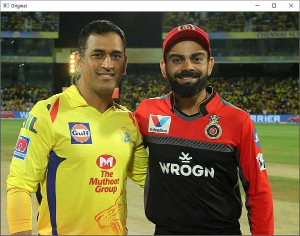
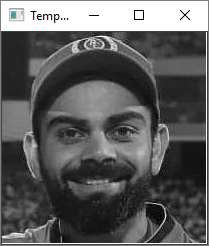
In an example below, an image having Indian cricketer Virat Kohlis face is used as a template to be matched with another image which depicts his photograph with another Indian cricketer M.S.Dhoni.
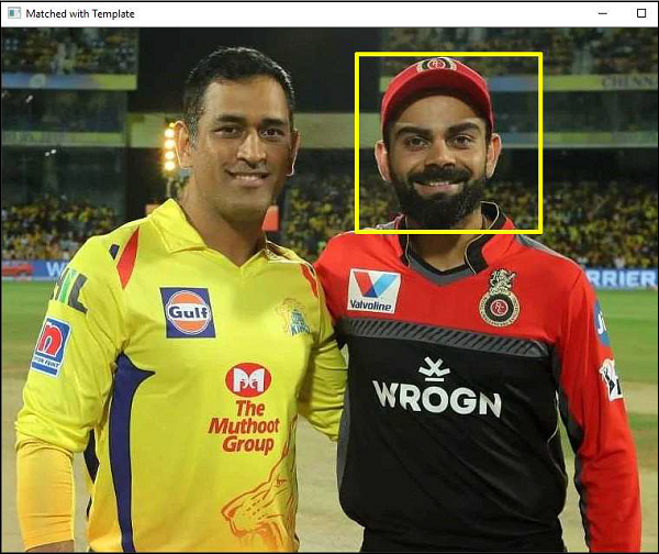
Following program uses a threshold value of 80% and draws a rectangle around the matching face −
import cv2
import numpy as np

img = cv2.imread('Dhoni-and-Virat.jpg',1)
cv2.imshow('Original',img)
gray = cv2.cvtColor(img, cv2.COLOR_BGR2GRAY)

template = cv2.imread('virat.jpg',0)
cv2.imshow('Template',template)
w,h = template.shape[0], template.shape[1]

matched = cv2.matchTemplate(gray,template,cv2.TM_CCOEFF_NORMED)
threshold = 0.8

loc = np.where( matched >= threshold)

for pt in zip(*loc[::-1]):
   cv2.rectangle(img, pt, (pt[0] + w, pt[1] + h), (0,255,255), 2)

cv2.imshow('Matched with Template',img)
Output
The original image, the template and matched image of the result as follows −
Original image
The template is as follows −
The image when matched with template is as follows −
OpenCV Python - Image Pyramids
Occasionally, we may need to convert an image to a size different than its original. For this, you either Upsize the image (zoom in) or Downsize it (zoom out).
An image pyramid is a collection of images (constructed from a single original image) successively down sampled a specified number of times.
The Gaussian pyramid is used to down sample images while the Laplacian pyramid reconstructs an up sampled image from an image lower in the pyramid with less resolution.
Consider the pyramid as a set of layers. The image is shown below −
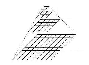
Image at the higher layer of the pyramid is smaller in size. To produce an image at the next layer in the Gaussian pyramid, we convolve a lower level image with a Gaussian kernel.
$$\frac{1}{16}\begin{bmatrix}1 & 4 & 6 & 4 & 1 \\4 & 16 & 24 & 16 & 4 \\6 & 24 & 36 & 24 & 6 \\4 & 16 & 24 & 16 & 4 \\1 & 4 & 6 & 4 & 1\end{bmatrix}$$
Now remove every even-numbered row and column. Resulting image will be 1/4th the area of its predecessor. Iterating this process on the original image produces the entire pyramid.
To make the images bigger, the columns filled with zeros. First, upsize the image to double the original in each dimension, with the new even rows and then perform a convolution with the kernel to approximate the values of the missing pixels.
The cv.pyrUp() function doubles the original size and cv.pyrDown() function decreases it to half.
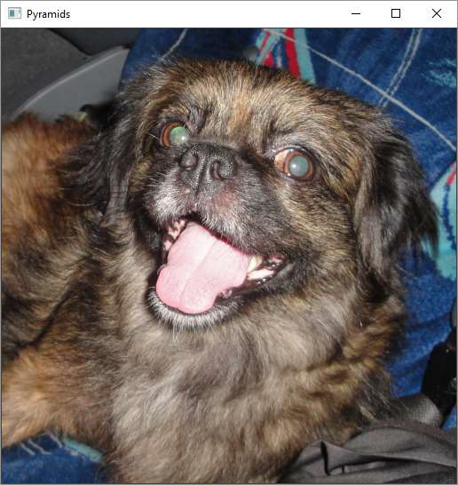
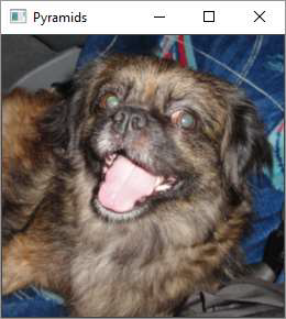
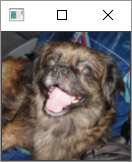
Example
Following program calls pyrUp() and pyrDown() functions depending on user input I or o respectively.
Note that when we reduce the size of an image, information of the image is lost. Once, we scale down and if we rescale it to the original size, we lose some information and the resolution of the new image is much lower than the original one.
import sys
import cv2 as cv

filename = 'chicky_512.png'

src = cv.imread(filename)

while 1:
   print ("press 'i' for zoom in 'o' for zoom out esc to stop")
   rows, cols, _channels = map(int, src.shape)
   cv.imshow('Pyramids', src)
   k = cv.waitKey(0)

   if k == 27:
      break

   elif chr(k) == 'i':
      src = cv.pyrUp(src, dstsize=(2 * cols, 2 * rows))

   elif chr(k) == 'o':
      src = cv.pyrDown(src, dstsize=(cols // 2, rows // 2))

cv.destroyAllWindows()
Output
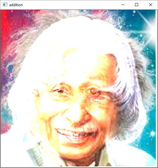
OpenCV Python - Image Addition
When an image is read by imread() function, the resultant image object is really a two or three dimensional matrix depending upon if the image is grayscale or RGB image.
Hence, cv2.add() functions add two image matrices and returns another image matrix.
Example
Following code reads two images and performs their binary addition −
kalam = cv2.imread('kalam.jpg')
einst = cv2.imread('einstein.jpg')
img = cv2.add(kalam, einst)
cv2.imshow('addition', img)
Result
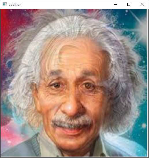
Instead of a linear binary addition, OpenCV has a addWeighted() function that performs weighted sum of two arrays. The command for the same is as follows
Cv2.addWeighted(src1, alpha, src2, beta, gamma)
Parameters
The parameters of the addWeighted() function are as follows −
- src1 − First input array.
- alpha − Weight of the first array elements.
- src2 − Second input array of the same size and channel number as first
- beta − Weight of the second array elements.
- gamma − Scalar added to each sum.
This function adds the images as per following equation −
$$\mathrm{g(x)=(1-\alpha)f_{0}(x)+\alpha f_{1}(x)}$$
The image matrices obtained in the above example are used to perform weighted sum.
By varying a from 0 -> 1, a smooth transition takes place from one image to another, so that they blend together.
First image is given a weight of 0.3 and the second image is given 0.7. The gamma factor is taken as 0.
The command for addWeighted() function is as follows −
img = cv2.addWeighted(kalam, 0.3, einst, 0.7, 0)
It can be seen that the image addition is smoother compared to binary addition.
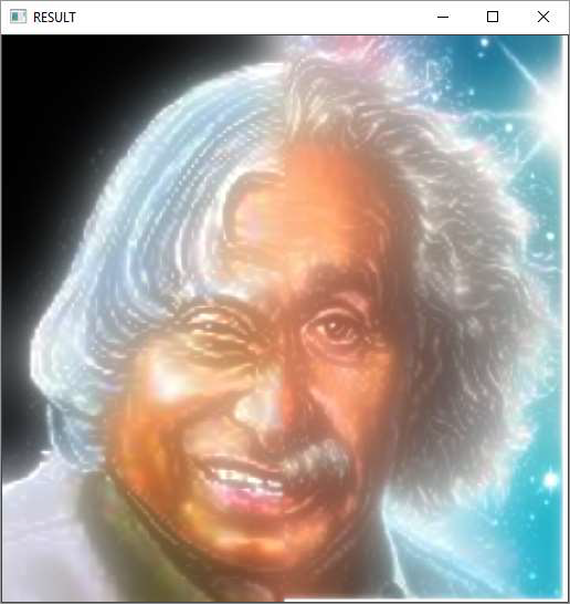
OpenCV Python - Image Blending with Pyramids
The discontinuity of images can be minimised by the use of image pyramids. This results in a seamless blended image.
Following steps are taken to achieve the final result −
First load the images and find Gaussian pyramids for both. The program for the same is as follows −
import cv2
import numpy as np,sys

kalam = cv2.imread('kalam.jpg')
einst = cv2.imread('einstein.jpg')
### generate Gaussian pyramid for first
G = kalam.copy()
gpk = [G]
for i in range(6):
   G = cv2.pyrDown(G)
   gpk.append(G)
# generate Gaussian pyramid for second
G = einst.copy()
gpe = [G]
for i in range(6):
   G = cv2.pyrDown(G)
   gpe.append(G)
From the Gaussian pyramids, obtain the respective Laplacian Pyramids. The program for the same is as follows −
# generate Laplacian Pyramid for first
lpk = [gpk[5]]
for i in range(5,0,-1):
   GE = cv2.pyrUp(gpk[i])
   L = cv2.subtract(gpk[i-1],GE)
   lpk.append(L)

# generate Laplacian Pyramid for second
lpe = [gpe[5]]
for i in range(5,0,-1):
   GE = cv2.pyrUp(gpe[i])
   L = cv2.subtract(gpe[i-1],GE)
   lpe.append(L)
Then, join the left half of the first image with the right half of second in each level of pyramids. The program for the same is as follows −
# Now add left and right halves of images in each level
LS = []
for la,lb in zip(lpk,lpe):
   rows,cols,dpt = la.shape
   ls = np.hstack((la[:,0:int(cols/2)], lb[:,int(cols/2):]))
   LS.append(ls)
Finally, reconstruct the image from this joint pyramid. The program for the same is given below −
ls_ = LS[0]
for i in range(1,6):
   ls_ = cv2.pyrUp(ls_)
   ls_ = cv2.add(ls_, LS[i])
   cv2.imshow('RESULT',ls_)
Output
The blended result should be as follows −
OpenCV Python - Fourier Transform
The Fourier Transform is used to transform an image from its spatial domain to its frequency domain by decomposing it into its sinus and cosines components.
In case of digital images, a basic gray scale image values usually are between zero and 255. Therefore, the Fourier Transform too needs to be a Discrete Fourier Transform (DFT). It is used to find the frequency domain.
Mathematically, Fourier Transform of a two dimensional image is represented as follows −
$$\mathrm{F(k,l)=\displaystyle\sum\limits_{i=0}^{N-1}\: \displaystyle\sum\limits_{j=0}^{N-1} f(i,j)\:e^{-i2\pi (\frac{ki}{N},\frac{lj}{N})}}$$
If the amplitude varies so fast in a short time, you can say it is a high frequency signal. If it varies slowly, it is a low frequency signal.
In case of images, the amplitude varies drastically at the edge points, or noises. So edges and noises are high frequency contents in an image. If there are no much changes in amplitude, it is a low frequency component.
OpenCV provides the functions cv.dft() and cv.idft() for this purpose.
cv.dft() performs a Discrete Fourier transform of a 1D or 2D floating-point array. The command for the same is as follows −
cv.dft(src, dst, flags)
Here,
- src − Input array that could be real or complex.
- dst − Output array whose size and type depends on the flags.
- flags − Transformation flags, representing a combination of the DftFlags.
cv.idft() calculates the inverse Discrete Fourier Transform of a 1D or 2D array. The command for the same is as follows −
cv.idft(src, dst, flags)
In order to obtain a discrete fourier transform, the input image is converted to np.float32 datatype. The transform obtained is then used to Shift the zero-frequency component to the center of the spectrum, from which magnitude spectrum is calculated.
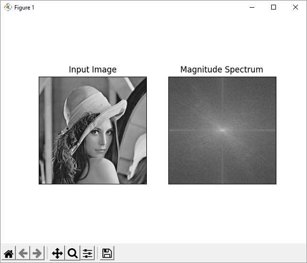
Example
Given below is the program using Matplotlib, we plot the original image and magnitude spectrum −
import numpy as np
import cv2 as cv
from matplotlib import pyplot as plt
img = cv.imread('lena.jpg',0)
dft = cv.dft(np.float32(img),flags = cv.DFT_COMPLEX_OUTPUT)
dft_shift = np.fft.fftshift(dft)
magnitude_spectrum = 20*np.log(cv.magnitude(dft_shift[:,:,0],dft_shift[:,:,1]))
plt.subplot(121),plt.imshow(img, cmap = 'gray')
plt.title('Input Image'), plt.xticks([]), plt.yticks([])
plt.subplot(122),plt.imshow(magnitude_spectrum, cmap = 'gray')
plt.title('Magnitude Spectrum'), plt.xticks([]), plt.yticks([])
plt.show()
Output
OpenCV Python - Capture Video from Camera
By using the VideoCapture() function in OpenCV library, it is very easy to capture a live stream from a camera on the OpenCV window.
This function needs a device index as the parameter. Your computer may have multiple cameras attached. They are enumerated by an index starting from 0 for built-in webcam. The function returns a VideoCapture object
cam = cv.VideoCapture(0)
After the camera is opened, we can read successive frames from it with the help of read() function
ret,frame = cam.read()
The read() function reads the next available frame and a return value (True/False). This frame is now rendered in desired color space with the cvtColor() function and displayed on the OpenCV window.
img = cv.cvtColor(frame, cv.COLOR_BGR2RGB)
# Display the resulting frame
cv.imshow('frame', img)
To capture the current frame to an image file, you can use imwrite() function.
cv2.imwrite(capture.png, img)
To save the live stream from camera to a video file, OpenCV provides a VideoWriter() function.
cv.VideoWriter( filename, fourcc, fps, frameSize)
The fourcc parameter is a standardized code for video codecs. OpenCV supports various codecs such as DIVX, XVID, MJPG, X264 etc. The fps anf framesize parameters depend on the video capture device.
The VideoWriter() function returns a VideoWrite stream object, to which the grabbed frames are successively written in a loop. Finally, release the frame and VideoWriter objects to finalize the creation of video.
Example
Following example reads live feed from built-in webcam and saves it to ouput.avi file.
import cv2 as cv
cam = cv.VideoCapture(0)
cc = cv.VideoWriter_fourcc(*'XVID')
file = cv.VideoWriter('output.avi', cc, 15.0, (640, 480))
if not cam.isOpened():
   print("error opening camera")
   exit()
while True:
   # Capture frame-by-frame
   ret, frame = cam.read()
   # if frame is read correctly ret is True
   if not ret:
      print("error in retrieving frame")
      break
   img = cv.cvtColor(frame, cv.COLOR_BGR2RGB)
   cv.imshow('frame', img)
   file.write(img)


   if cv.waitKey(1) == ord('q'):
      break

cam.release()
file.release()
cv.destroyAllWindows()
OpenCV Python - Play Video from File
The VideoCapture() function can also retrieve frames from a video file instead of a camera. Hence, we have only replaced the camera index with the video files name to be played on the OpenCV window.
video=cv2.VideoCapture(file)
While this should be enough to start rendering a video file, if it is accompanied by sound. The sound will not play along. For this purpose, you will need to install the ffpyplayer module.
FFPyPlayer
FFPyPlayer is a python binding for the FFmpeg library for playing and writing media files. To install, use pip installer utility by using the following command.
pip3 install ffpyplayer
The get_frame() method of the MediaPlayer object in this module returns the audio frame which will play along with each frame read from the video file.
Following is the complete code for playing a video file along with its audio −
import cv2

from ffpyplayer.player import MediaPlayer
file="video.mp4"

video=cv2.VideoCapture(file)
player = MediaPlayer(file)
while True:
   ret, frame=video.read()
   audio_frame, val = player.get_frame()
   if not ret:
      print("End of video")
      break
   if cv2.waitKey(1) == ord("q"):
      break
   cv2.imshow("Video", frame)
   if val != 'eof' and audio_frame is not None:
      #audio
      img, t = audio_frame
video.release()
cv2.destroyAllWindows()
OpenCV Python - Extract Images from Video
A video is nothing but a sequence of frames and each frame is an image. By using OpenCV, all the frames that compose a video file can be extracted by executing imwrite() function till the end of video.
The cv2.read() function returns the next available frame. The function also gives a return value which continues to be true till the end of stream. Here, a counter is incremented inside the loop and used as a file name.
Following program demonstrates how to extract images from the video −
import cv2
import os

cam = cv2.VideoCapture("video.avi")

frameno = 0
while(True):
   ret,frame = cam.read()
   if ret:
      # if video is still left continue creating images
      name = str(frameno) + '.jpg'
      print ('new frame captured...' + name)

      cv2.imwrite(name, frame)
      frameno += 1
   else:
      break

cam.release()
cv2.destroyAllWindows()
OpenCV Python - Video from Images
In the previous chapter, we have used the VideoWriter() function to save the live stream from a camera as a video file. To stitch multiple images into a video, we shall use the same function.
First, ensure that all the required images are in a folder. Pythons glob() function in the built-in glob module builds an array of images so that we can iterate through it.
Read the image object from the images in the folder and append to an image array.
Following program explains how to stitch multiple images in a video −
import cv2
import numpy as np
import glob

img_array = []
for filename in glob.glob('*.png'):
   img = cv2.imread(filename)
   height, width, layers = img.shape
   size = (width,height)
   img_array.append(img)
The create a video stream by using VideoWriter() function to write the contents of the image array to it. Given below is the program for the same.
out = cv2.VideoWriter('video.avi',cv2.VideoWriter_fourcc(*'DIVX'), 15, size)

for i in range(len(img_array)):
   out.write(img_array[i])
out.release()
You should find the file named video.avi in the current folder.
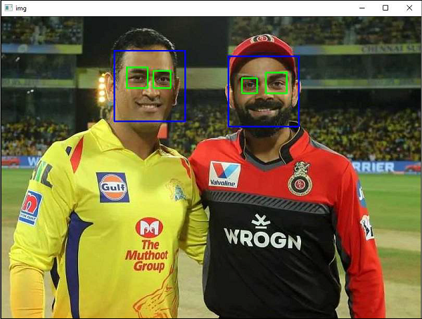
OpenCV Python - Face Detection
OpenCV uses Haar feature-based cascade classifiers for the object detection. It is a machine learning based algorithm, where a cascade function is trained from a lot of positive and negative images. It is then used to detect objects in other images. The algorithm uses the concept of Cascade of Classifiers.
Pretrained classifiers for face, eye etc. can be downloaded from https://github.com
For the following example, download and copy haarcascade_frontalface_default.xml and haarcascade_eye.xml from this URL. Then, load our input image to be used for face detection in grayscale mode.
The DetectMultiScale() method of CascadeClassifier class detects objects in the input image. It returns the positions of detected faces as in the form of Rectangle and its dimensions (x,y,w,h). Once we get these locations, we can use it for eye detection since eyes are always on the face!
Example
The complete code for face detection is as follows −
import numpy as np
import cv2

face_cascade = cv2.CascadeClassifier('haarcascade_frontalface_default.xml')
eye_cascade = cv2.CascadeClassifier('haarcascade_eye.xml')

img = cv2.imread('Dhoni-and-virat.jpg')
gray = cv2.cvtColor(img, cv2.COLOR_BGR2GRAY)
faces = face_cascade.detectMultiScale(gray, 1.3, 5)
for (x,y,w,h) in faces:
   img = cv2.rectangle(img,(x,y),(x+w,y+h),(255,0,0),2)
   roi_gray = gray[y:y+h, x:x+w]
   roi_color = img[y:y+h, x:x+w]
   eyes = eye_cascade.detectMultiScale(roi_gray)
   for (ex,ey,ew,eh) in eyes:
      cv2.rectangle(roi_color,(ex,ey),(ex+ew,ey+eh),(0,255,0),2)

cv2.imshow('img',img)
cv2.waitKey(0)
cv2.destroyAllWindows()
Output
You will get rectangles drawn around faces in the input image as shown below −
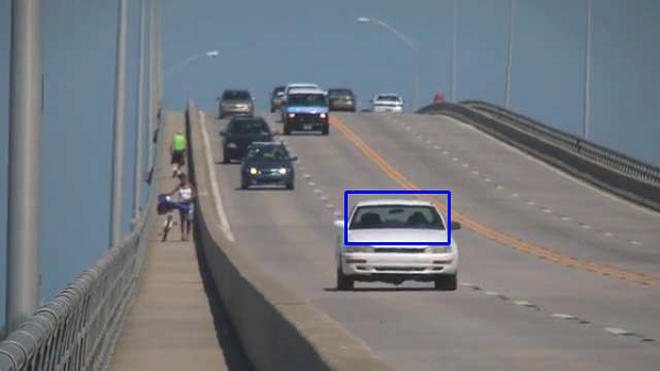
OpenCV Python - Meanshift and Camshift
In this chapter, let us learn about the meanshift and the camshift in the OpenCV-Python. First, let us understand what is meanshift.
Meanshift
The mean shift algorithm identifies places in the data set with a high concentration of data points, or clusters. The algorithm places a kernel at each data point and sums them together to make a Kernel Density Estimation (KDE).
The KDE will have places with a high and low data point density, respectfully. Meanshift is a very useful method to keep the track of a particular object inside a video.
Every instance of the video is checked in the form of pixel distribution in that frame. An initial window as region of interest (ROI) is generally a square or a circle. For this, the positions are specified by hardcoding and the area of maximum pixel distribution is identified.
The ROI window moves towards the region of maximum pixel distribution as the video runs. The direction of movement depends upon the difference between the center of our tracking window and the centroid of all the k-pixels inside that window.
In order to use Meanshift in OpenCV, first, find the histogram (of which, only Hue is considered) of our target and can back project its target on each frame for calculation of Meanshift. We also need to provide an initial location of the ROI window.
We repeatedly calculate the back projection of the histogram and calculate the Meanshift to get the new position of track window. Later on, we draw a rectangle using its dimensions on the frame.
Functions
The openCV functions used in the program are −
cv.calcBackProject() − Calculates the back projection of a histogram.
cv.meanShift() − Back projection of the object histogram using initial search window and Stop criteria for the iterative search algorithm.
Example
Here is the example program of Meanshift −
import numpy as np
import cv2 as cv

cap = cv.VideoCapture('traffic.mp4')

ret,frame = cap.read()

# dimensions of initial location of window
x, y, w, h = 300, 200, 100, 50
tracker = (x, y, w, h)

region = frame[y:y+h, x:x+w]
hsv_reg = cv.cvtColor(region, cv.COLOR_BGR2HSV)
mask = cv.inRange(hsv_reg, np.array((0., 60.,32.)), np.array((180.,255.,255.)))
reg_hist = cv.calcHist([hsv_reg],[0],mask,[180],[0,180])
cv.normalize(reg_hist,reg_hist,0,255,cv.NORM_MINMAX)

# Setup the termination criteria
criteria = ( cv.TERM_CRITERIA_EPS | cv.TERM_CRITERIA_COUNT, 10, 1 )

while(1):
   ret, frame = cap.read()

   if ret == True:
      hsv = cv.cvtColor(frame, cv.COLOR_BGR2HSV)
      dst = cv.calcBackProject([hsv],[0],reg_hist,[0,180],1)

      # apply meanshift
      ret, tracker = cv.meanShift(dst, tracker, criteria)

      # Draw it on image
      x,y,w,h = tracker
      img = cv.rectangle(frame, (x,y), (x+w,y+h), 255,2)
      cv.imshow('img',img)

      k = cv.waitKey(30) & 0xff
      if k==115:
         cv.imwrite('capture.png', img)
      if k == 27:
         break
As the program is run, the Meanshift algorithm moves our window to the new location with maximum density.
Output
Heres a snapshot of moving window −
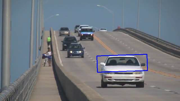
Camshift
One of the disadvantages of Meanshift algorithm is that the size of the tracking window remains the same irrespective of the object's distance from the camera. Also, the window will track the object only if it is in the region of that object. So, we must do manual hardcoding of the window and it should be done carefully.
The solution to these problems is given by CAMshift (stands for Continuously Adaptive Meanshift). Once meanshift converges, the Camshift algorithm updates the size of the window such that the tracking window may change in size or even rotate to better correlate to the movements of the tracked object.
In the following code, instead of meanshift() function, the camshift() function is used.
First, it finds an object center using meanShift and then adjusts the window size and finds the optimal rotation. The function returns the object position, size, and orientation. The position is drawn on the frame by using polylines() draw function.
Example
Instead of Meanshift() function in earlier program, use CamShift() function as below −
# apply camshift
ret, tracker = cv.CamShift(dst, tracker, criteria)
pts = cv.boxPoints(ret)
pts = np.int0(pts)
img = cv.polylines(frame,[pts],True, 255,2)
cv.imshow('img',img)
Output
One snapshot of the result of modified program showing rotated rectangle of the tracking window is as follows −
OpenCV Python - Feature Detection
In the context of image processing, features are mathematical representations of key areas in an image. They are the vector representations of the visual content from an image.
Features make it possible to perform mathematical operations on them. Various computer vision applications include object detection, motion estimation, segmentation, image alignment etc.
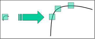
Prominent features in any image include edges, corners or parts of an image. OpenCV supports Haris corner detection and Shi-Tomasi corner detection algorithms. OpenCV library also provides functionality to implement SIFT (Scale-Invariant Feature Transform), SURF(Speeded-Up Robust Features) and FAST algorithm for corner detection.
Harris and Shi-Tomasi algorithms are rotation-invariant. Even if the image is rotated, we can find the same corners. But when an image is scaled up, a corner may not be a corner if the image. The figure given below depicts the same.
D.Lowe's new algorithm, Scale Invariant Feature Transform (SIFT) extracts the key points and computes its descriptors.
This is achieved by following steps −
- Scale-space Extrema Detection.
- Keypoint Localization.
- Orientation Assignment.
- Keypoint Descriptor.
- Keypoint Matching.
As far as implementation of SIFT in OpenCV is concerned, it starts from loading an image and converting it into grayscale. The cv.SHIFT_create() function creates a SIFT object.
Example
Calling its detect() method obtains key points which are drawn on top of the original image. Following code implements this procedure
import numpy as np
import cv2 as cv
img = cv.imread('home.jpg')
gray= cv.cvtColor(img,cv.COLOR_BGR2GRAY)
sift = cv.SIFT_create()
kp = sift.detect(gray,None)
img=cv.drawKeypoints(gray,kp,img)
cv.imwrite('keypoints.jpg',img)
Output
The original image and the one with keypoints drawn are shown below −
This is an original image.
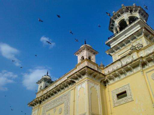
An image given below is the one with keypoints −
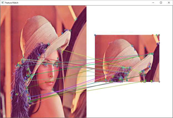
OpenCV Python - Feature Matching
OpenCV provides two techniques for feature matching. Brute force matching and FLANN matcher technique.
Example
Following example uses brute-force method
import numpy as np
import cv2

img1 = cv2.imread('lena.jpg')
img2 = cv2.imread('lena-test.jpg')

# Convert it to grayscale
img1_bw = cv2.cvtColor(img1,cv2.COLOR_BGR2GRAY)
img2_bw = cv2.cvtColor(img2, cv2.COLOR_BGR2GRAY)

orb = cv2.ORB_create()

queryKeypoints, queryDescriptors = orb.detectAndCompute(img1_bw,None)
trainKeypoints, trainDescriptors = orb.detectAndCompute(img2_bw,None)

matcher = cv2.BFMatcher()
matches = matcher.match(queryDescriptors,trainDescriptors)

img = cv2.drawMatches(img1, queryKeypoints,
img2, trainKeypoints, matches[:20],None)

img = cv2.resize(img, (1000,650))

cv2.imshow("Feature Match", img)
Output
OpenCV Python - Digit Recognition with KNN
KNN which stands for K-Nearest Neighbour is a Machine Learning algorithm based on Supervised Learning. It tries to put a new data point into the category that is most similar to the available categories. All the available data is classified into distinct categories and a new data point is put in one of them based on the similarity.
The KNN algorithm works on following principle −
- Choose preferably an odd number as K for the number of neighbours to be checked.
- Calculate their Euclidean distance.
- Take the K nearest neighbors as per the calculated Euclidean distance.
- count the number of the data points in each category.
- Category with maximum data points is the category in which the new data point is classified.
As an example of implementation of KNN algorithm using OpenCV, we shall use the following image digits.png consisting of 5000 images of handwritten digits, each of 20X20 pixels.
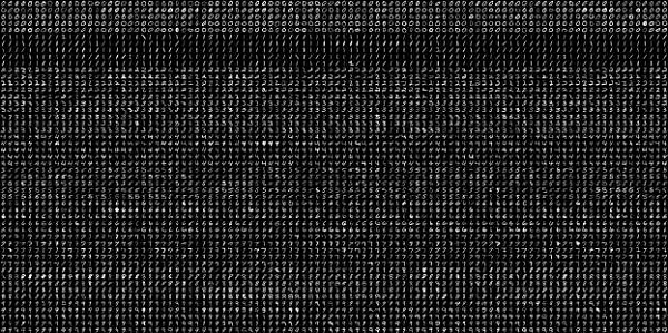
First task is to split this image into 5000 digits. This is our feature set. Convert it to a NumPy array. The program is given below −
import numpy as np
import cv2

image = cv2.imread('digits.png')
gray = cv2.cvtColor(image, cv2.COLOR_BGR2GRAY)

fset=[]
for i in np.vsplit(gray,50):
   x=np.hsplit(i,100)
   fset.append(x)

NP_array = np.array(fset)
Now we divide this data in training set and testing set, each of size (2500,20x20) as follows −
trainset = NP_array[:,:50].reshape(-1,400).astype(np.float32)
testset = NP_array[:,50:100].reshape(-1,400).astype(np.float32)
Next, we have to create 10 different labels for each digit, as shown below −
k = np.arange(10)
train_labels = np.repeat(k,250)[:,np.newaxis]
test_labels = np.repeat(k,250)[:,np.newaxis]
We are now in a position to start the KNN classification. Create the classifier object and train the data.
knn = cv2.ml.KNearest_create()
knn.train(trainset, cv2.ml.ROW_SAMPLE, train_labels)
Choosing the value of k as 3, obtain the output of the classifier.
ret, output, neighbours, distance = knn.findNearest(testset, k = 3)
Compare the output with test labels to check the performance and accuracy of the classifier.
The program shows an accuracy of 91.64% in detecting the handwritten digit accurately.
result = output==test_labels
correct = np.count_nonzero(result)
accuracy = (correct*100.0)/(output.size)
print(accuracy)
