How to highlight whole numbers in Excel?

In the article, the users are going to highlight the whole numbers in Microsoft Excel. There are several features in the excel sheet including conditional formatting, and format cells that the users have to fill any type of color according to their needs. The users can use the formula for changing cell values in the new formatting rule dialog box. The users can use select the range in which they want to fill the color in any cell.

To highlight whole numbers in Excel

Step 1

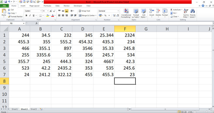
Deliberate the excel sheet with the data. First, open the excel sheet and create the data one by one. In this sheet, type any type of number like decimal or numerical numbers A1:F7 which the users need to highlight the numerical or non-decimal numbers in the list as shown below.

Step 2

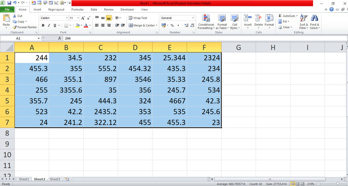
In the excel sheet, the created data is displayed. Place the cursor in the cell A1 and select all the cells which the users inserted the random numbers one by one.

Step 3

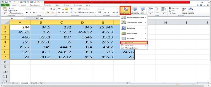
After selecting all the data in the sheet, place the cursor in the ribbon. In the ribbon, there are many tabs included in the top corner. Place the cursor in the Home tab and click on the tab that has many options included. On Home tab, place the cursor and click on the drop-down menu of Conditional Formatting. On this tab, click on the New Rule tab that opens the dialog box as shown below.

Step 4

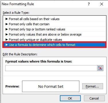
In the dialog box, there are the rules included one by one. Select and click on the rule Use a formula to determine which cells to format that enables the drop-box like this.

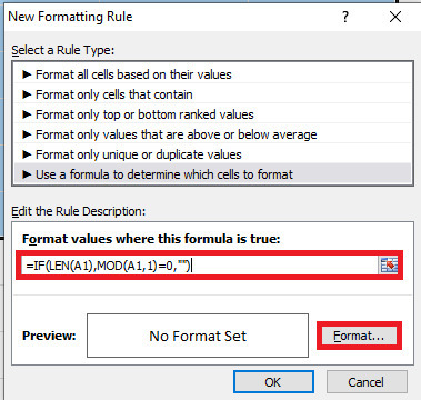
Step 5

In the dialog box, there is the input type and place the cursor on it. Now, enter the formula =IF(LEN(A1),MOD(A1,1)=0,””) to highlight the whole numerical numbers. In the dialog box, place the cursor and click on the Format button that opens a new dialog box Format Cells that has the Fill tab. In the dialog box of Format Cells, there are the tabs included. Now, click on the Fill tab that displays the color theme like this.

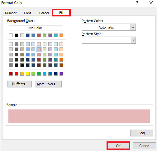
Step 6

In the dialog box, choose any color in the color theme as shown which the users want to highlight whole numerical numbers then click on the ok button that closes the dialog box of Format Cells. After closing the Format Cells dialog box, the New Formatting Rule dialog box will display as shown below.

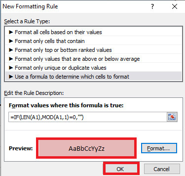
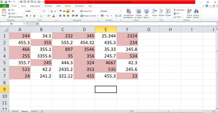
Step 7

In the dialog box, click on the ok button that will close the New Formatting dialog box. After closing the dialog boxes, it will highlight whole numbers with the selected color from color theme randomly as shown below.

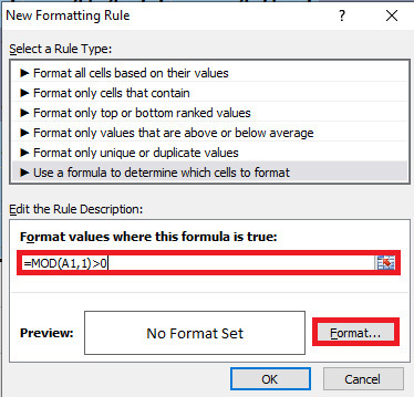
Step 8

After selecting the number list, again open the dialog box and enter the formula =MOD(A1,1)>0 to highlight the whole decimal numbers. In the dialog box, place the cursor and click on the Format button that opens a new dialog box Format Cells that has the Fill tab. In the dialog box of Format Cells, there are the tabs included. Now, click on the Fill tab that displays the color theme like this.

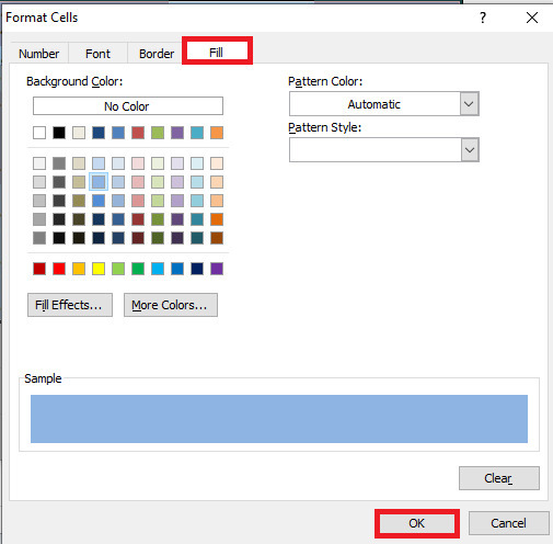
Step 9

In the dialog box, choose any color in the color theme as shown which the users want to highlight only decimal numbers then click on the ok button that closes the dialog box of Format Cells. After closing the Format Cells dialog box, the New Formatting Rule dialog box will display as shown below.

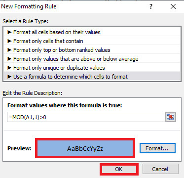
Step 10

In the dialog box, click on the ok button that will close the New Formatting dialog box. After closing the dialog boxes, it will highlight whole decimal numbers with the selected color from color theme randomly as shown below.

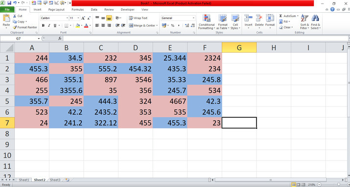
Conclusion

The users utilized an easy instance to display how can highlight the whole numbers like numerical and decimal numbers with different colors randomly. The users used the necessary tabs which are included in the ribbon. The users have to practice the essential options from the ribbon and modify the data according to their needs.