How to highlight rows based on multiple cell values in excel?

In the article, the users are going to highlight the rows based on multiple cell values in Microsoft Excel. There are several features in the Excel sheet including conditional formatting, and format cells that the users have to fill any type of color according to their needs. The users can use conditional formatting for highlighting the multiple values in the row. The users can use select the conditional format to highlight the row one by one in which they want to fill the color in any cell.

To highlight rows based on multiple cell values in excel

Step 1

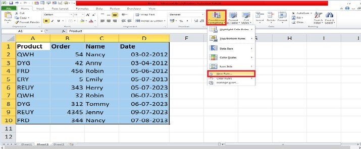
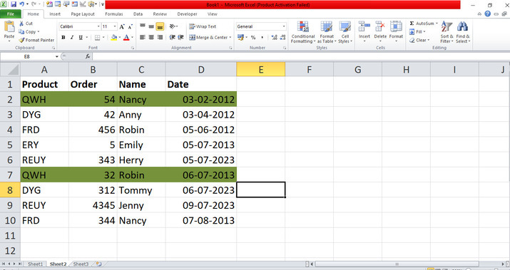
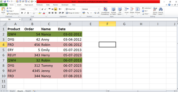
Deliberate the Excel sheet with the data. First, open the Excel sheet and create the data one by one. In this sheet, type the product and its order with name and date randomly and it will create data that the users have to highlight as shown below.

Step 2

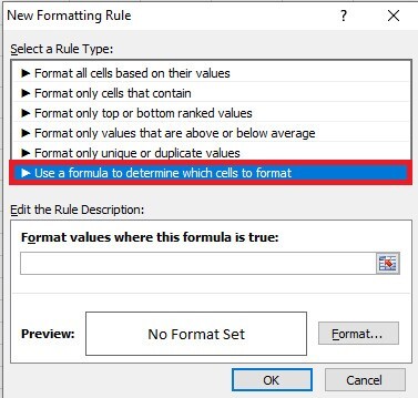
In the Excel sheet, the created data is displayed. After creating the rows based on multiple values in the list, place the cursor in cell A2 and select all the cells in which the users inserted the data one by one. After selecting all the data in the sheet, place the cursor in the ribbon. On the Home tab, place the cursor and click on the drop-down menu of Conditional Formatting. On this tab, there are many options included. Click on the New Rule button that opens the New Formatting Rule dialog box as shown below.

Step 3

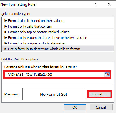
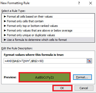
In the dialog box, there are the rules included one by one. Select and click on the rule Use a formula to determine which cells to format that enables the drop-box like this.

Step 4

In the dialog box, there is the input type and place the cursor on it. Now, enter the formula =AND($A2=”QWH”, $B2>50) to highlight same product and the value must be greater than 50 in the order field as shown below.

Step 5

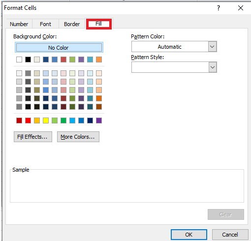
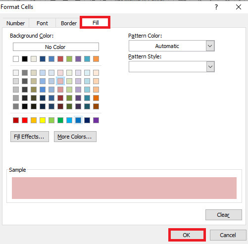
In the dialog box, place the cursor and click on the Format button that opens a new dialog box Format Cells that has the Fill tab. In the dialog box of Format Cells, there are the tabs included. Now, click on the Fill tab that displays the color theme like this.

Step 6

In the dialog box, choose any color in the color theme as shown which the users want to highlight only same products with the value which is greater than 50 then click on the ok button that closes the dialog box of Format Cells. After closing the Format Cells dialog box, the New Formatting Rule dialog box will display as shown below.

Step 7

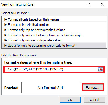
In the dialog box, there is the input type and place the cursor on it. Now, enter the formula to highlight the same product and the value must be greater than 300 in the order field. In the dialog box, place the cursor and click on the Format button that opens a new dialog box Format Cells which has the Fill tab. After closing the Format Cells dialog box, the New Formatting Rule dialog box will display as shown below.

Conclusion

The users utilized an easy instance to highlight the multiple cell values with different colors randomly. With the help of conditional formatting, the conditions are to be set to highlight the rows based on a certain condition. The step-by-step explanations are depicted in this article to understand the problem statement clearly. The users used the necessary tabs which are included in the ribbon. The users have to practice the essential options from the ribbon and modify the data according to their needs.