
Article Categories
- All Categories
-
 Data Structure
-
 Networking
-
 RDBMS
RDBMS
-
 Operating System
-
 Java
Java
-
 MS Excel
-
 iOS
iOS
-
 HTML
HTML
-
 CSS
CSS
-
 Android
-
 Python
-
 C Programming
-
 C++
C++
-
 C#
C#
-
 MongoDB
-
 MySQL
MySQL
-
 Javascript
-
 PHP
PHP
-
 Economics & Finance
How to Extract All Duplicates from a Column in Excel
To extract duplicate values from a column in Excel, you can use the COUNTIF formula combined with conditional formatting. First, apply the formula "=COUNTIF(A:A,A1)>1" to identify duplicate values in a new column. Then, use conditional formatting to highlight the cells that meet the condition. This will visually highlight the duplicate values. Additionally, you can filter the column by the duplicate values or use the Advanced Filter feature to extract them to a new column. These methods help you quickly identify and extract duplicate values in Excel.
Steps to Extract Duplicate Values from a Column in Excel
Step 1:Open your Excel file First, open the Excel file that you want to work with. If you don't have an Excel file yet, create one by clicking on the "New Workbook" button on the Excel start page.
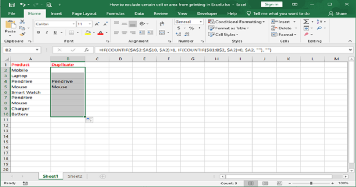
Step 2:Create Sample data with the data in column A. Create another column as Duplicate and select the cell where the result to display.

Step 3:Enter the formula as:
Example
=IF(COUNTIF($A$2:$A$10, $A2)>1, IF(COUNTIF($B1:B$2, $A2)=0, $A2, ""), "")

Note: Adjust the range $A$1:$A$10 to match the range of your data. The formula checks if the count of a value in column A is greater than 1, and if so, it checks if the value has already been listed in column B. If it hasn't, the value is displayed; otherwise, an empty cell is shown.
Press enter to view duplicate value.
Step 4: Drag the formula in cell B1 down to cover all the cells in column B corresponding to your data range. This will populate column B with unique duplicate values.
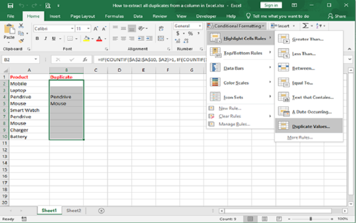
Step 5: Go to the "Home" tab in the Excel ribbon. Click on "Conditional Formatting" in the "Styles" group. Select "Highlight Cells Rules" from the dropdown menu. Choose "Duplicate Values" from the submenu.
Step 6: In the "Duplicate Values" dialog box, you can choose how to format the duplicates. For example, you can select a highlight color or a custom format.
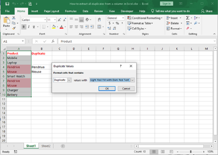
Step 7: Click "OK" to apply the conditional formatting. Now, Excel will highlight all the duplicate values in the selected column or range with the formatting you chose. This makes it easy to visually identify and analyse the duplicate values in your spreadsheet.

Conclusion
To extract duplicate values from a column in Excel and display them as unique in another column, follow these steps. First, open your Excel file and navigate to the sheet with the data. In column B, enter the provided formula, which checks for duplicate values in column A. Adjust the range to match your data. Drag the formula down to cover all the cells in column B. This populates column B with unique duplicate values.
Next, select the range of cells in column B containing the unique duplicates. Apply conditional formatting by going to the "Conditional Formatting" option in the "Styles" group under the "Home" tab. Select "Highlight Cells Rules" from the dropdown menu. Choose "Duplicate Values" from the submenu. Click "OK" to apply the conditional formatting.
You will have successfully identified and displayed the duplicate values as unique in another column. The conditional formatting visually highlights the unique duplicates, making them easily identifiable. This method helps organize and analyze data by isolating and distinguishing duplicate values within an Excel spreadsheet.

4K+ Views
