ggplot2 - Working with Axes

---

---

When we speak about axes in graphs, it is all about x and y axis which is represented in two dimensional manner. In this chapter, we will focus about two datasets “Plantgrowth” and “Iris” dataset which is commonly used by data scientists.

Implementing axes in Iris dataset

We will use the following steps to work on x and y axes using ggplot2 package of R.

It is always important to load the library to get the functionalities of package.

# Load ggplot
library(ggplot2)

# Read in dataset
data(iris)

Creating the plot points

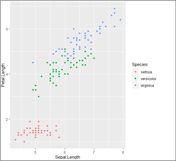
Like discussed in the previous chapter, we will create a plot with points in it. In other words, it is defined as scattered plot.

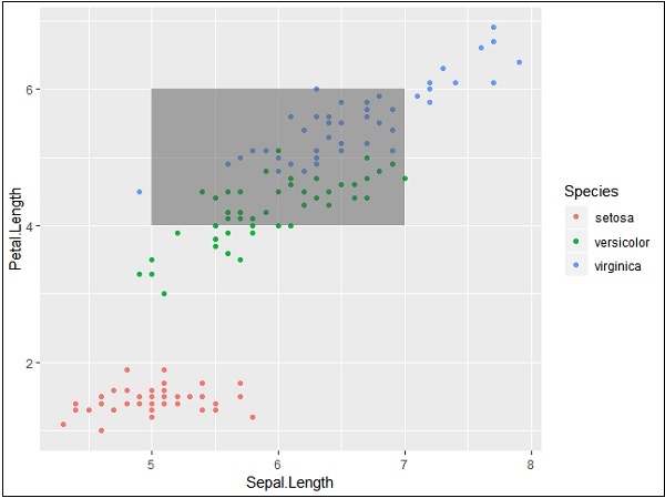
# Plot
p <- ggplot(iris, aes(Sepal.Length, Petal.Length, colour=Species)) + geom_point()
p

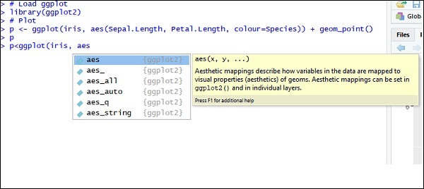
Now let us understand the functionality of aes which mentions the mapping structure of “ggplot2”. Aesthetic mappings describe the variable structure which is needed for plotting and the data which should be managed in individual layer format.

The output is given below −

Highlight and tick marks

Plot the markers with mentioned co-ordinates of x and y axes as mentioned below. It includes adding text, repeating text, highlighting particular area and adding segment as follows −

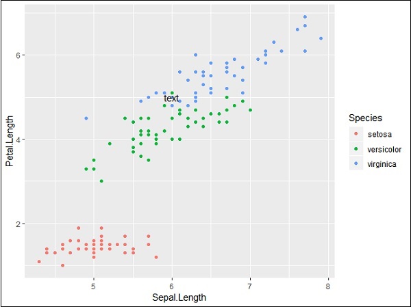
# add text
p + annotate("text", x = 6, y = 5, label = "text")

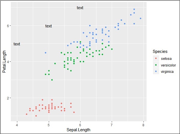
# add repeat
p + annotate("text", x = 4:6, y = 5:7, label = "text")

# highlight an area
p + annotate("rect", xmin = 5, xmax = 7, ymin = 4, ymax = 6, alpha = .5)

# segment
p + annotate("segment", x = 5, xend = 7, y = 4, yend = 5, colour = "black")

The output generated for adding text is given below −

Repeating particular text with mentioned co-ordinates generates the following output. The text is generated with x co-ordinates from 4 to 6 and y co-ordinates from 5 to 7 −

The segmentation and highlighting of particular area output is given below −

PlantGrowth Dataset

Now let us focus on working with other dataset called “Plantgrowth” and the step which is needed is given below.

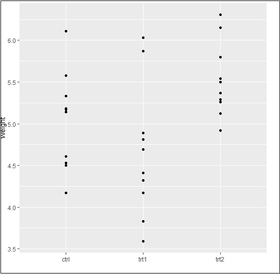
Call for the library and check out the attributes of “Plantgrowth”. This dataset includes results from an experiment to compare yields (as measured by dried weight of plants) obtained under a control and two different treatment conditions.

> PlantGrowth
  weight group
1 4.17 ctrl
2 5.58 ctrl
3 5.18 ctrl
4 6.11 ctrl
5 4.50 ctrl
6 4.61 ctrl
7 5.17 ctrl
8 4.53 ctrl
9 5.33 ctrl
10 5.14 ctrl
11 4.81 trt1
12 4.17 trt1
13 4.41 trt1
14 3.59 trt1
15 5.87 trt1
16 3.83 trt1
17 6.03 trt1

Adding attributes with axes

Try plotting a simple plot with required x and y axis of the graph as mentioned below −

> bp <- ggplot(PlantGrowth, aes(x=group, y=weight)) +
+    geom_point()
> bp

The output generated is given below −

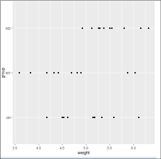
Finally, we can swipe x and y axes as per our requirement with basic function as mentioned below −

> bp <- ggplot(PlantGrowth, aes(x=group, y=weight)) +
+    geom_point()
> bp

Basically, we can use many properties with aesthetic mappings to get working with axes using ggplot2.