
Article Categories
- All Categories
-
 Data Structure
-
 Networking
-
 RDBMS
RDBMS
-
 Operating System
-
 Java
Java
-
 MS Excel
-
 iOS
iOS
-
 HTML
HTML
-
 CSS
CSS
-
 Android
-
 Python
-
 C Programming
-
 C++
C++
-
 C#
C#
-
 MongoDB
-
 MySQL
MySQL
-
 Javascript
-
 PHP
PHP
-
 Economics & Finance
Exploratory Data Analysis on Iris Dataset
Introduction
In Machine Learning and Data Science Exploratory Data Analysis is the process of examining a data set and summarizing its main characteristics about it. It may include visual methods to better represent those characteristics or have a general understanding of the dataset. It is a very essential step in a Data Science lifecycle, often consuming a certain time.
In this article, we are going to see some of the characteristics of the Iris dataset through Exploratory Data Analysis.
The Iris Dataset
The Iris Dataset is very simple often referred to as the Hello World. The dataset has 4 features of three different species of flowers namely Iris setosa, Iris virginica, and Iris versicolor. These features are sepal length, sepal width, petal length, and petal width. There are 150 data points in the dataset, 50 data points for each species.
EDA on Iris Dataset
First, let's load the dataset from the CSV file "iris_csv.csv" using pandas and have a general overview of it.
The dataset can be downloaded from the below link.
https://datahub.io/machine-learning/iris/r/iris.csv
Code Implementation
Example 1
<div class="code-mirror  language-python" contenteditable="plaintext-only" spellcheck="false" style="outline: none; overflow-wrap: break-word; overflow-y: auto; white-space: pre-wrap;"><span class="token keyword">import</span> pandas <span class="token keyword">as</span> pd
<span class="token keyword">import</span> numpy <span class="token keyword">as</span> np
<span class="token keyword">import</span> seaborn <span class="token keyword">as</span> sns
<span class="token keyword">import</span> matplotlib<span class="token punctuation">.</span>pyplot <span class="token keyword">as</span> plt
<span class="token operator">%</span>matplotlib inline

df <span class="token operator">=</span> pd<span class="token punctuation">.</span>read_csv<span class="token punctuation">(</span><span class="token string">"/content/iris_csv.csv"</span><span class="token punctuation">)</span>
df<span class="token punctuation">.</span>head<span class="token punctuation">(</span><span class="token punctuation">)</span>
</div>
sepallength |
sepalwidth |
petallength |
petalwidth |
class |
|
|---|---|---|---|---|---|
0 |
5.1 |
3.5 |
1.4 |
0.2 |
Iris-setosa |
1 |
4.9 |
3.0 |
1.4 |
0.2 |
Iris-setosa |
3 |
4.6 |
3.1 |
1.5 |
0.2 |
Iris-setosa |
4 |
5.0 |
3.6 |
1.4 |
0.2 |
Iris-seto |
Example 2
<div class="code-mirror  language-python" contenteditable="plaintext-only" spellcheck="false" style="outline: none; overflow-wrap: break-word; overflow-y: auto; white-space: pre-wrap;">df<span class="token punctuation">.</span>info<span class="token punctuation">(</span><span class="token punctuation">)</span>

RangeIndex<span class="token punctuation">:</span> <span class="token number">150</span> entries<span class="token punctuation">,</span> <span class="token number">0</span> to <span class="token number">149</span>
Data columns <span class="token punctuation">(</span>total <span class="token number">5</span> columns<span class="token punctuation">)</span><span class="token punctuation">:</span>
 <span class="token comment">#   Column       Non-Null Count  Dtype  </span>
<span class="token operator">-</span><span class="token operator">-</span><span class="token operator">-</span>  <span class="token operator">-</span><span class="token operator">-</span><span class="token operator">-</span><span class="token operator">-</span><span class="token operator">-</span><span class="token operator">-</span>       <span class="token operator">-</span><span class="token operator">-</span><span class="token operator">-</span><span class="token operator">-</span><span class="token operator">-</span><span class="token operator">-</span><span class="token operator">-</span><span class="token operator">-</span><span class="token operator">-</span><span class="token operator">-</span><span class="token operator">-</span><span class="token operator">-</span><span class="token operator">-</span><span class="token operator">-</span>  <span class="token operator">-</span><span class="token operator">-</span><span class="token operator">-</span><span class="token operator">-</span><span class="token operator">-</span>
 <span class="token number">0</span>   sepallength  <span class="token number">150</span> non<span class="token operator">-</span>null    float64
 <span class="token number">1</span>   sepalwidth   <span class="token number">150</span> non<span class="token operator">-</span>null    float64
 <span class="token number">2</span>   petallength  <span class="token number">150</span> non<span class="token operator">-</span>null    float64
 <span class="token number">3</span>   petalwidth   <span class="token number">150</span> non<span class="token operator">-</span>null    float64
 <span class="token number">4</span>   <span class="token keyword">class</span>        <span class="token class-name">150</span> non<span class="token operator">-</span>null    <span class="token builtin">object</span>
dtypes<span class="token punctuation">:</span> float64<span class="token punctuation">(</span><span class="token number">4</span><span class="token punctuation">)</span><span class="token punctuation">,</span> <span class="token builtin">object</span><span class="token punctuation">(</span><span class="token number">1</span><span class="token punctuation">)</span>
memory usage<span class="token punctuation">:</span> <span class="token number">6.0</span><span class="token operator">+</span> KB
df<span class="token punctuation">.</span>shape

<span class="token punctuation">(</span><span class="token number">150</span><span class="token punctuation">,</span> <span class="token number">5</span><span class="token punctuation">)</span>


<span class="token comment">## Statistics about dataset</span>
df<span class="token punctuation">.</span>describe<span class="token punctuation">(</span><span class="token punctuation">)</span>
</div>
sepallength |
sepalwidth |
petallength |
petalwidth |
|
|---|---|---|---|---|
count |
150.000000 |
150.000000 |
150.000000 |
150.000000 |
mean |
5.843333 |
3.054000 |
3.758667 |
1.198667 |
std |
0.828066 |
0.433594 |
1.764420 |
0.763161 |
min |
4.300000 |
2.000000 |
1.000000 |
0.100000 |
25% |
5.100000 |
2.800000 |
1.600000 |
0.300000 |
50% |
5.800000 |
3.000000 |
4.350000 |
1.300000 |
max |
7.900000 |
4.400000 |
6.900000 |
2.500000 |
Example 3
<div class="code-mirror  language-python" contenteditable="plaintext-only" spellcheck="false" style="outline: none; overflow-wrap: break-word; overflow-y: auto; white-space: pre-wrap;"><span class="token comment">## checking for null values</span>

df<span class="token punctuation">.</span>isnull<span class="token punctuation">(</span><span class="token punctuation">)</span><span class="token punctuation">.</span><span class="token builtin">sum</span><span class="token punctuation">(</span><span class="token punctuation">)</span>

sepallength    <span class="token number">0</span>
sepalwidth     <span class="token number">0</span>
petallength    <span class="token number">0</span>
petalwidth     <span class="token number">0</span>
<span class="token keyword">class</span>          <span class="token class-name">0</span>
dtype<span class="token punctuation">:</span> int64

<span class="token comment">## Univariate analysis</span>
df<span class="token punctuation">.</span>groupby<span class="token punctuation">(</span><span class="token string">'class'</span><span class="token punctuation">)</span><span class="token punctuation">.</span>agg<span class="token punctuation">(</span><span class="token punctuation">[</span><span class="token string">'mean'</span><span class="token punctuation">,</span> <span class="token string">'median'</span><span class="token punctuation">]</span><span class="token punctuation">)</span>  <span class="token comment"># passing a list of recognized strings</span>
df<span class="token punctuation">.</span>groupby<span class="token punctuation">(</span><span class="token string">'class'</span><span class="token punctuation">)</span><span class="token punctuation">.</span>agg<span class="token punctuation">(</span><span class="token punctuation">[</span>np<span class="token punctuation">.</span>mean<span class="token punctuation">,</span> np<span class="token punctuation">.</span>median<span class="token punctuation">]</span><span class="token punctuation">)</span>
</div>
| sepallength | sepalwidth | petallength | petalwidth | |||||
|---|---|---|---|---|---|---|---|---|
| mean | median | mean | median | mean | median | mean | median | |
| class | ||||||||
| Iris?setosa | 5.006 | 5.0 | 3.418 | 3.4 | 1.464 | 1.50 | 0.244 | 0.2 |
| Iris?versicolor | 5.936 | 5.9 | 2.770 | 2.8 | 4.260 | 4.35 | 1.326 | 1.3 |
| Iris?virginica | 6.588 | 6.5 | 2.974 | 3.0 | 5.552 | 5.55 | 2.026 | 2.0 |
Example 4
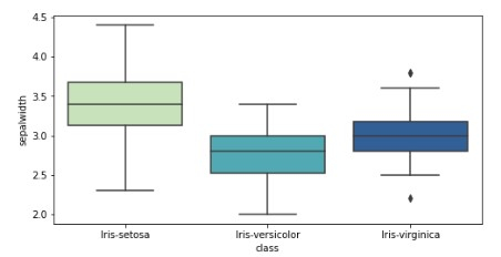
<div class="code-mirror  language-python" contenteditable="plaintext-only" spellcheck="false" style="outline: none; overflow-wrap: break-word; overflow-y: auto; white-space: pre-wrap;"><span class="token comment">## Box plot </span>
plt<span class="token punctuation">.</span>figure<span class="token punctuation">(</span>figsize<span class="token operator">=</span><span class="token punctuation">(</span><span class="token number">8</span><span class="token punctuation">,</span><span class="token number">4</span><span class="token punctuation">)</span><span class="token punctuation">)</span>
sns<span class="token punctuation">.</span>boxplot<span class="token punctuation">(</span>x<span class="token operator">=</span><span class="token string">'class'</span><span class="token punctuation">,</span>y<span class="token operator">=</span><span class="token string">'sepalwidth'</span><span class="token punctuation">,</span>data<span class="token operator">=</span>df <span class="token punctuation">,</span>palette<span class="token operator">=</span><span class="token string">'YlGnBu'</span><span class="token punctuation">)</span>
</div>
Example 5
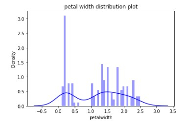
<div class="code-mirror  language-python" contenteditable="plaintext-only" spellcheck="false" style="outline: none; overflow-wrap: break-word; overflow-y: auto; white-space: pre-wrap;"><span class="token comment">## Distribution of particular species</span>
sns<span class="token punctuation">.</span>distplot<span class="token punctuation">(</span>a<span class="token operator">=</span>df<span class="token punctuation">[</span><span class="token string">'petalwidth'</span><span class="token punctuation">]</span><span class="token punctuation">,</span> bins<span class="token operator">=</span><span class="token number">40</span><span class="token punctuation">,</span> color<span class="token operator">=</span><span class="token string">'b'</span><span class="token punctuation">)</span>
plt<span class="token punctuation">.</span>title<span class="token punctuation">(</span><span class="token string">'petal width distribution plot'</span><span class="token punctuation">)</span>
</div>
Example 6
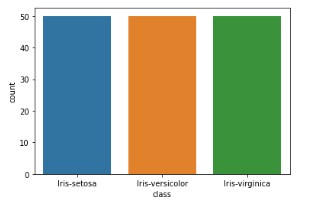
<div class="code-mirror  language-python" contenteditable="plaintext-only" spellcheck="false" style="outline: none; overflow-wrap: break-word; overflow-y: auto; white-space: pre-wrap;"><span class="token comment">## count of number of observation of each species</span>

sns<span class="token punctuation">.</span>countplot<span class="token punctuation">(</span>x<span class="token operator">=</span><span class="token string">'class'</span><span class="token punctuation">,</span>data<span class="token operator">=</span>df<span class="token punctuation">)</span>
</div>
Example 7
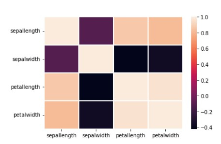
<div class="code-mirror  language-python" contenteditable="plaintext-only" spellcheck="false" style="outline: none; overflow-wrap: break-word; overflow-y: auto; white-space: pre-wrap;"><span class="token comment">## Correlation map using a heatmap matrix</span>

sns<span class="token punctuation">.</span>heatmap<span class="token punctuation">(</span>df<span class="token punctuation">.</span>corr<span class="token punctuation">(</span><span class="token punctuation">)</span><span class="token punctuation">,</span> linecolor<span class="token operator">=</span><span class="token string">'white'</span><span class="token punctuation">,</span> linewidths<span class="token operator">=</span><span class="token number">1</span><span class="token punctuation">)</span>
</div>
Example 8
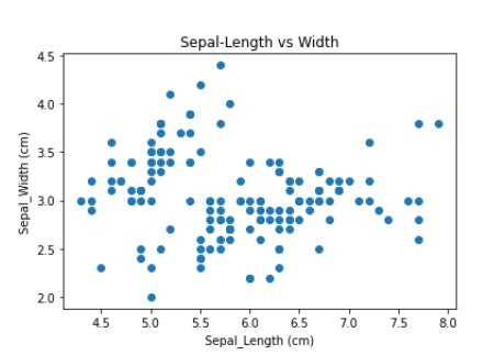
<div class="code-mirror  language-python" contenteditable="plaintext-only" spellcheck="false" style="outline: none; overflow-wrap: break-word; overflow-y: auto; white-space: pre-wrap;"><span class="token comment">## Multivariate analysis - analyis between two or more variable or features</span>
<span class="token comment">## Scatter plot to see the relation between two or more features like sepal length, petal length,etc</span>
axis <span class="token operator">=</span> plt<span class="token punctuation">.</span>axes<span class="token punctuation">(</span><span class="token punctuation">)</span>

axis<span class="token punctuation">.</span>scatter<span class="token punctuation">(</span>df<span class="token punctuation">.</span>sepallength<span class="token punctuation">,</span> df<span class="token punctuation">.</span>sepalwidth<span class="token punctuation">)</span>

axis<span class="token punctuation">.</span><span class="token builtin">set</span><span class="token punctuation">(</span>xlabel<span class="token operator">=</span><span class="token string">'Sepal_Length (cm)'</span><span class="token punctuation">,</span>
   ylabel<span class="token operator">=</span><span class="token string">'Sepal_Width (cm)'</span><span class="token punctuation">,</span>
   title<span class="token operator">=</span><span class="token string">'Sepal-Length vs Width'</span><span class="token punctuation">)</span><span class="token punctuation">;</span>
</div>
Example 9
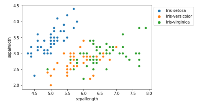
<div class="code-mirror  language-python" contenteditable="plaintext-only" spellcheck="false" style="outline: none; overflow-wrap: break-word; overflow-y: auto; white-space: pre-wrap;">sns<span class="token punctuation">.</span>scatterplot<span class="token punctuation">(</span>x<span class="token operator">=</span><span class="token string">'sepallength'</span><span class="token punctuation">,</span> y<span class="token operator">=</span><span class="token string">'sepalwidth'</span><span class="token punctuation">,</span> hue<span class="token operator">=</span><span class="token string">'class'</span><span class="token punctuation">,</span> data<span class="token operator">=</span>df<span class="token punctuation">,</span>
plt<span class="token punctuation">.</span>show<span class="token punctuation">(</span><span class="token punctuation">)</span>
</div>
Example 10
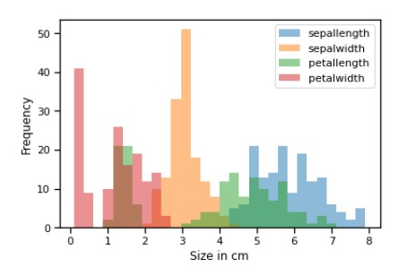
<div class="code-mirror  language-python" contenteditable="plaintext-only" spellcheck="false" style="outline: none; overflow-wrap: break-word; overflow-y: auto; white-space: pre-wrap;"><span class="token comment">## From the above graph we can see that</span>
<span class="token comment"># Iris-virginica has a longer sepal length while Iris-setosa has larger sepal width</span>
<span class="token comment"># For setosa sepal width is more than sepal length</span>
<span class="token comment">## Below is the Frequency histogram plot of all features</span>
axis <span class="token operator">=</span> df<span class="token punctuation">.</span>plot<span class="token punctuation">.</span>hist<span class="token punctuation">(</span>bins<span class="token operator">=</span><span class="token number">30</span><span class="token punctuation">,</span> alpha<span class="token operator">=</span><span class="token number">0.5</span><span class="token punctuation">)</span>
axis<span class="token punctuation">.</span>set_xlabel<span class="token punctuation">(</span><span class="token string">'Size in cm'</span><span class="token punctuation">)</span><span class="token punctuation">;</span>
</div>
Example 11
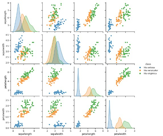
<div class="code-mirror  language-python" contenteditable="plaintext-only" spellcheck="false" style="outline: none; overflow-wrap: break-word; overflow-y: auto; white-space: pre-wrap;"><span class="token comment"># From the above graph we can see that sepalwidth is longer than any other feature followed by petalwidth</span>
<span class="token comment">## examining correlation</span>
sns<span class="token punctuation">.</span>pairplot<span class="token punctuation">(</span>df<span class="token punctuation">,</span> hue<span class="token operator">=</span><span class="token string">'class'</span><span class="token punctuation">)</span>
</div>
Example 12
<div class="code-mirror  language-python" contenteditable="plaintext-only" spellcheck="false" style="outline: none; overflow-wrap: break-word; overflow-y: auto; white-space: pre-wrap;">figure<span class="token punctuation">,</span> ax <span class="token operator">=</span> plt<span class="token punctuation">.</span>subplots<span class="token punctuation">(</span><span class="token number">2</span><span class="token punctuation">,</span> <span class="token number">2</span><span class="token punctuation">,</span> figsize<span class="token operator">=</span><span class="token punctuation">(</span><span class="token number">8</span><span class="token punctuation">,</span><span class="token number">8</span><span class="token punctuation">)</span><span class="token punctuation">)</span>

ax<span class="token punctuation">[</span><span class="token number">0</span><span class="token punctuation">,</span><span class="token number">0</span><span class="token punctuation">]</span><span class="token punctuation">.</span>set_title<span class="token punctuation">(</span><span class="token string">"sepallength"</span><span class="token punctuation">)</span>
ax<span class="token punctuation">[</span><span class="token number">0</span><span class="token punctuation">,</span><span class="token number">0</span><span class="token punctuation">]</span><span class="token punctuation">.</span>hist<span class="token punctuation">(</span>df<span class="token punctuation">[</span><span class="token string">'sepallength'</span><span class="token punctuation">]</span><span class="token punctuation">,</span> bins<span class="token operator">=</span><span class="token number">8</span><span class="token punctuation">)</span>

ax<span class="token punctuation">[</span><span class="token number">0</span><span class="token punctuation">,</span><span class="token number">1</span><span class="token punctuation">]</span><span class="token punctuation">.</span>set_title<span class="token punctuation">(</span><span class="token string">"sepalwidth"</span><span class="token punctuation">)</span>
ax<span class="token punctuation">[</span><span class="token number">0</span><span class="token punctuation">,</span><span class="token number">1</span><span class="token punctuation">]</span><span class="token punctuation">.</span>hist<span class="token punctuation">(</span>df<span class="token punctuation">[</span><span class="token string">'sepalwidth'</span><span class="token punctuation">]</span><span class="token punctuation">,</span> bins<span class="token operator">=</span><span class="token number">6</span><span class="token punctuation">)</span><span class="token punctuation">;</span>

ax<span class="token punctuation">[</span><span class="token number">1</span><span class="token punctuation">,</span><span class="token number">0</span><span class="token punctuation">]</span><span class="token punctuation">.</span>set_title<span class="token punctuation">(</span><span class="token string">"petallength"</span><span class="token punctuation">)</span>
ax<span class="token punctuation">[</span><span class="token number">1</span><span class="token punctuation">,</span><span class="token number">0</span><span class="token punctuation">]</span><span class="token punctuation">.</span>hist<span class="token punctuation">(</span>df<span class="token punctuation">[</span><span class="token string">'petallength'</span><span class="token punctuation">]</span><span class="token punctuation">,</span> bins<span class="token operator">=</span><span class="token number">5</span><span class="token punctuation">)</span><span class="token punctuation">;</span>

ax<span class="token punctuation">[</span><span class="token number">1</span><span class="token punctuation">,</span><span class="token number">1</span><span class="token punctuation">]</span><span class="token punctuation">.</span>set_title<span class="token punctuation">(</span><span class="token string">"petalwidth"</span><span class="token punctuation">)</span>
ax<span class="token punctuation">[</span><span class="token number">1</span><span class="token punctuation">,</span><span class="token number">1</span><span class="token punctuation">]</span><span class="token punctuation">.</span>hist<span class="token punctuation">(</span>df<span class="token punctuation">[</span><span class="token string">'petalwidth'</span><span class="token punctuation">]</span><span class="token punctuation">,</span> bins<span class="token operator">=</span><span class="token number">5</span><span class="token punctuation">)</span><span class="token punctuation">;</span>
</div>
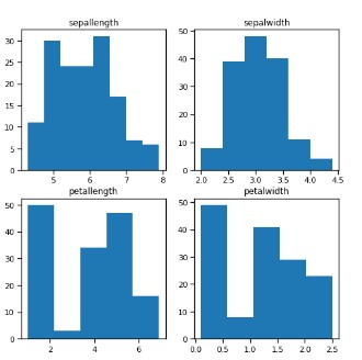
Example 13
<div class="code-mirror  language-python" contenteditable="plaintext-only" spellcheck="false" style="outline: none; overflow-wrap: break-word; overflow-y: auto; white-space: pre-wrap;"><span class="token comment"># From the above plot we can see that -</span>
<span class="token comment"># - Sepal length highest freq lies between 5.5 cm to 6 cm which is 30-35 cm</span>
<span class="token comment"># - Petal length highest freq lies between 1 cm to 2 cm which is 50 cm</span>
<span class="token comment"># - Sepal width highest freq lies between 3 cm to 3.5 cm which is 70 cm</span>
<span class="token comment"># - Petal width highest freq lies between 0 cm to 0.5 cm which is 40-45 cm</span>
</div>
Conclusion
Exploratory Data Analysis is extremely used by both Data Scientists and Analysts. It tells a lot about the characteristics of the given data, its distribution, and how it can be useful.

6K+ Views
