- DIP - Home
- DIP - Image Processing Introduction
- DIP - Signal and System Introduction
- DIP - History of Photography
- DIP - Applications and Usage
- DIP - Concept of Dimensions
- DIP - Image Formation on Camera
- DIP - Camera Mechanism
- DIP - Concept of Pixel
- DIP - Perspective Transformation
- DIP - Concept of Bits Per Pixel
- DIP - Types of Images
- DIP - Color Codes Conversion
- DIP - Grayscale to RGB Conversion
- DIP - Concept of Sampling
- DIP - Pixel Resolution
- DIP - Concept of Zooming
- DIP - Zooming methods
- DIP - Spatial Resolution
- DIP - Pixels Dots and Lines per inch
- DIP - Gray Level Resolution
- DIP - Concept of Quantization
- DIP - ISO Preference curves
- DIP - Concept of Dithering
- DIP - Histograms Introduction
- DIP - Brightness and Contrast
- DIP - Image Transformations
- DIP - Histogram Sliding
- DIP - Histogram Stretching
- DIP - Introduction to Probability
- DIP - Histogram Equalization
- DIP - Gray Level Transformations
- DIP - Concept of convolution
- DIP - Concept of Masks
- DIP - Concept of Blurring
- DIP - Concept of Edge Detection
- DIP - Prewitt Operator
- DIP - Sobel operator
- DIP - Robinson Compass Mask
- DIP - Krisch Compass Mask
- DIP - Laplacian Operator
- DIP - Frequency Domain Analysis
- DIP - Fourier series and Transform
- DIP - Convolution theorm
- DIP - High Pass vs Low Pass Filters
- DIP - Introduction to Color Spaces
- DIP - JPEG compression
- DIP - Optical Character Recognition
- DIP - Computer Vision and Graphics
Digital Image Processing - Concept of Quantization
We have introduced quantization in our tutorial of signals and system. We are formally going to relate it with digital images in this tutorial. Lets discuss first a little bit about quantization.
Digitizing a Signal
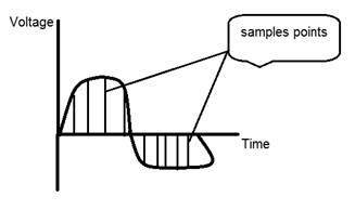
As we have seen in the previous tutorials, that digitizing an analog signal into a digital, requires two basic steps. Sampling and quantization. Sampling is done on x axis. It is the conversion of x axis (infinite values) to digital values.
The below figure shows sampling of a signal.
Sampling with relation to digital images
The concept of sampling is directly related to zooming. The more samples you take, the more pixels, you get. Oversampling can also be called as zooming. This has been discussed under sampling and zooming tutorial.
But the story of digitizing a signal does not end at sampling too, there is another step involved which is known as Quantization.
What is Quantization?
Quantization is opposite to sampling. It is done on y axis. When you are quantizing an image, you are actually dividing a signal into quanta(partitions).
On the x axis of the signal, are the co-ordinate values, and on the y axis, we have amplitudes. So digitizing the amplitudes is known as Quantization.
Here how it is done
You can see in this image, that the signal has been quantified into three different levels. That means that when we sample an image, we actually gather a lot of values, and in quantization, we set levels to these values. This can be more clear in the image below.
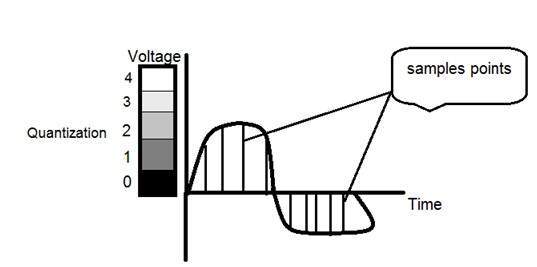
In the figure shown in sampling, although the samples has been taken, but they were still spanning vertically to a continuous range of gray level values. In the figure shown above, these vertically ranging values have been quantized into 5 different levels or partitions. Ranging from 0 black to 4 white. This level could vary according to the type of image you want.
The relation of quantization with gray levels has been further discussed below.
Relation of Quantization with gray level resolution:
The quantized figure shown above has 5 different levels of gray. It means that the image formed from this signal, would only have 5 different colors. It would be a black and white image more or less with some colors of gray. Now if you were to make the quality of the image more better, there is one thing you can do here. Which is, to increase the levels, or gray level resolution up. If you increase this level to 256, it means you have an gray scale image. Which is far better then simple black and white image.
Now 256, or 5 or what ever level you choose is called gray level. Remember the formula that we discussed in the previous tutorial of gray level resolution which is,
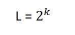
We have discussed that gray level can be defined in two ways. Which were these two.
- Gray level = number of bits per pixel (BPP).(k in the equation)
- Gray level = number of levels per pixel.
In this case we have gray level is equal to 256. If we have to calculate the number of bits, we would simply put the values in the equation. In case of 256levels, we have 256 different shades of gray and 8 bits per pixel, hence the image would be a gray scale image.
Reducing Gray Level
Now we will reduce the gray levels of the image to see the effect on the image.
For example
Lets say you have an image of 8bpp, that has 256 different levels. It is a grayscale image and the image looks something like this.
256 Gray Levels
Now we will start reducing the gray levels. We will first reduce the gray levels from 256 to 128.
128 Gray Levels
There is not much effect on an image after decrease the gray levels to its half. Lets decrease some more.
64 Gray Levels
Still not much effect, then lets reduce the levels more.
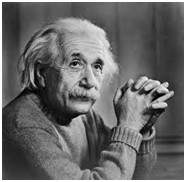
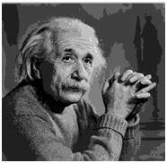
32 Gray Levels

Surprised to see, that there is still some little effect. May be its due to reason, that it is the picture of Einstein, but lets reduce the levels more.
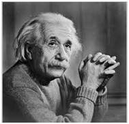
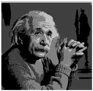
16 Gray Levels
Boom here, we go, the image finally reveals, that it is effected by the levels.
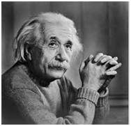
8 Gray Levels
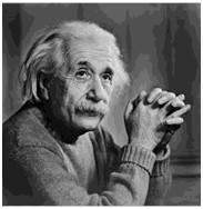
4 Gray Levels
Now before reducing it, further two 2 levels, you can easily see that the image has been distorted badly by reducing the gray levels. Now we will reduce it to 2 levels, which is nothing but a simple black and white level. It means the image would be simple black and white image.
2 Gray Levels
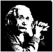
Thats the last level we can achieve, because if reduce it further, it would be simply a black image, which can not be interpreted.
Contouring
There is an interesting observation here, that as we reduce the number of gray levels, there is a special type of effect start appearing in the image, which can be seen clear in 16 gray level picture. This effect is known as Contouring.
Iso Preference Curves
The answer to this effect, that why it appears, lies in Iso preference curves. They are discussed in our next tutorial of Contouring and Iso preference curves.