- DIP - Home
- DIP - Image Processing Introduction
- DIP - Signal and System Introduction
- DIP - History of Photography
- DIP - Applications and Usage
- DIP - Concept of Dimensions
- DIP - Image Formation on Camera
- DIP - Camera Mechanism
- DIP - Concept of Pixel
- DIP - Perspective Transformation
- DIP - Concept of Bits Per Pixel
- DIP - Types of Images
- DIP - Color Codes Conversion
- DIP - Grayscale to RGB Conversion
- DIP - Concept of Sampling
- DIP - Pixel Resolution
- DIP - Concept of Zooming
- DIP - Zooming methods
- DIP - Spatial Resolution
- DIP - Pixels Dots and Lines per inch
- DIP - Gray Level Resolution
- DIP - Concept of Quantization
- DIP - ISO Preference curves
- DIP - Concept of Dithering
- DIP - Histograms Introduction
- DIP - Brightness and Contrast
- DIP - Image Transformations
- DIP - Histogram Sliding
- DIP - Histogram Stretching
- DIP - Introduction to Probability
- DIP - Histogram Equalization
- DIP - Gray Level Transformations
- DIP - Concept of convolution
- DIP - Concept of Masks
- DIP - Concept of Blurring
- DIP - Concept of Edge Detection
- DIP - Prewitt Operator
- DIP - Sobel operator
- DIP - Robinson Compass Mask
- DIP - Krisch Compass Mask
- DIP - Laplacian Operator
- DIP - Frequency Domain Analysis
- DIP - Fourier series and Transform
- DIP - Convolution theorm
- DIP - High Pass vs Low Pass Filters
- DIP - Introduction to Color Spaces
- DIP - JPEG compression
- DIP - Optical Character Recognition
- DIP - Computer Vision and Graphics
Digital Image Processing - Histogram Equalization
We have already seen that contrast can be increased using histogram stretching. In this tutorial we will see that how histogram equalization can be used to enhance contrast.
Before performing histogram equalization, you must know two important concepts used in equalizing histograms. These two concepts are known as PMF and CDF.
They are discussed in our tutorial of PMF and CDF. Please visit them in order to successfully grasp the concept of histogram equalization.
Histogram Equalization
Histogram equalization is used to enhance contrast. It is not necessary that contrast will always be increase in this. There may be some cases were histogram equalization can be worse. In that cases the contrast is decreased.
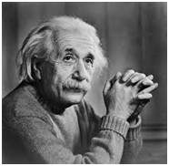
Lets start histogram equalization by taking this image below as a simple image.
Image
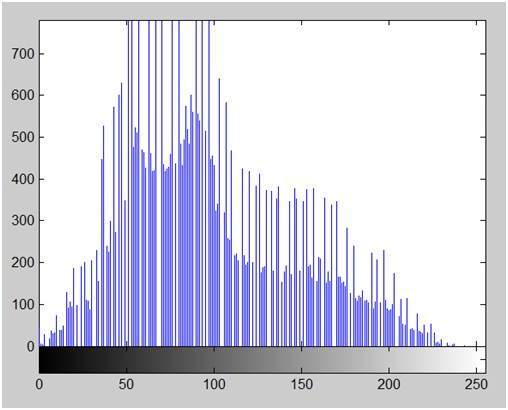
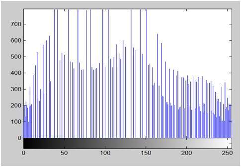
Histogram of this image
The histogram of this image has been shown below.
Now we will perform histogram equalization to it.
PMF
First we have to calculate the PMF (probability mass function) of all the pixels in this image. If you donot know how to calculate PMF, please visit our tutorial of PMF calculation.
CDF
Our next step involves calculation of CDF (cumulative distributive function). Again if you donot know how to calculate CDF , please visit our tutorial of CDF calculation.
Calculate CDF according to gray levels
Lets for instance consider this , that the CDF calculated in the second step looks like this.
| Gray Level Value | CDF |
|---|---|
| 0 | 0.11 |
| 1 | 0.22 |
| 2 | 0.55 |
| 3 | 0.66 |
| 4 | 0.77 |
| 5 | 0.88 |
| 6 | 0.99 |
| 7 | 1 |
Then in this step you will multiply the CDF value with (Gray levels (minus) 1) .
Considering we have an 3 bpp image. Then number of levels we have are 8. And 1 subtracts 8 is 7. So we multiply CDF by 7. Here what we got after multiplying.
| Gray Level Value | CDF | CDF * (Levels-1) |
|---|---|---|
| 0 | 0.11 | 0 |
| 1 | 0.22 | 1 |
| 2 | 0.55 | 3 |
| 3 | 0.66 | 4 |
| 4 | 0.77 | 5 |
| 5 | 0.88 | 6 |
| 6 | 0.99 | 6 |
| 7 | 1 | 7 |
Now we have is the last step, in which we have to map the new gray level values into number of pixels.
Lets assume our old gray levels values has these number of pixels.
| Gray Level Value | Frequency |
|---|---|
| 0 | 2 |
| 1 | 4 |
| 2 | 6 |
| 3 | 8 |
| 4 | 10 |
| 5 | 12 |
| 6 | 14 |
| 7 | 16 |
Now if we map our new values to , then this is what we got.
| Gray Level Value | New Gray Level Value | Frequency |
|---|---|---|
| 0 | 0 | 2 |
| 1 | 1 | 4 |
| 2 | 3 | 6 |
| 3 | 4 | 8 |
| 4 | 5 | 10 |
| 5 | 6 | 12 |
| 6 | 6 | 14 |
| 7 | 7 | 16 |
Now map these new values you are onto histogram, and you are done.
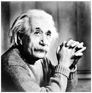
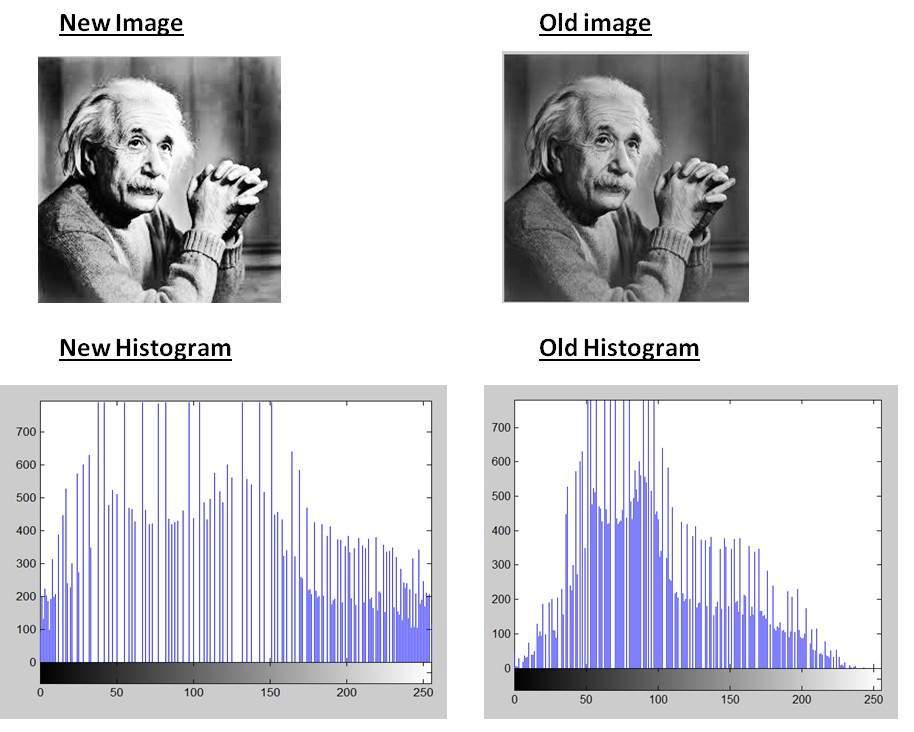
Lets apply this technique to our original image. After applying we got the following image and its following histogram.
Histogram Equalization Image
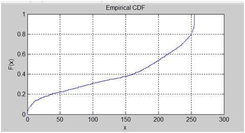
Cumulative Distributive function of this image
Histogram Equalization histogram
Comparing both the histograms and images
Conclusion
As you can clearly see from the images that the new image contrast has been enhanced and its histogram has also been equalized. There is also one important thing to be note here that during histogram equalization the overall shape of the histogram changes, where as in histogram stretching the overall shape of histogram remains same.