Create a gauss pulse using scipy.signal gausspulse

What are the uses of gauss pulse?

Gaussian pulses are widely used in signal processing, particularly in radar, sonar, and communications. This pulse is a pulse that has a Gaussian shape in the time domain, which makes it useful for detecting small signals that may be obscured by noise. In this tutorial, we will explore how to generate a Gaussian pulse using the scipy.signal.gausspulse function.

What is a Gaussian Pulse?

Gaussian pulses are a type of function that has a Gaussian-shaped envelope in the time domain. The Gaussian function is a bell-shaped curve that is symmetrical around its peak. It has a characteristic width or deviation, which determines how quickly the curve falls off as you move away from the peak.

Gaussian pulses are commonly used for communication, optics, and acoustics applications. They are known for their excellent time and frequency localization, which makes them ideal for detecting small signals that may be hidden in noise.

Prerequisites

Before we dive into the task few things should is expected to be installed onto your system

List of recommended settings −

• pip install scipy,numpy.

• It is expected that the user will have access to any standalone IDE such as VS-Code, PyCharm, Atom or Sublime text.

• Even online Python compilers can also be used such as Kaggle.com, Google Cloud platform or any other will do.

• Updated version of Python. At the time of writing the article I have used 3.10.9 version.

• Knowledge of the use of Jupyter notebook.

• Knowledge and application of virtual environment would be beneficial but not required.

• It is also expected that the person will have a good understanding of physics and signal processing concepts.

Creating a Gaussian Pulse using scipy.signal.gausspulse

The scipy.signal.gausspulse function can be used to generate a Gaussian pulse. The function has the following signature −

scipy.signal.gausspulse(t, fc, bw, return_padded=True, tpr=None, sym=True)

• t − time sampling vector

• fc − frequency of the center of the pulse

• bw − fractional bandwidth of the pulse

• return_padded − if True, pad the data to the nearest power of 2

• tpr − time-bandwidth product of the pulse

• sym − if True, generates a symmetric pulse

Each subsection of the signature explained

• t − time sampling vector

• This parameter specifies the time interval over which the pulse is defined. It is usually an array of equally spaced time samples that cover the duration of the pulse.

• fc − frequency of the center of the pulse

• This parameter specifies the center frequency of the pulse. The pulse is centered at this frequency, and the width of the pulse determines its bandwidth.

• bw − fractional bandwidth of the pulse

• This parameter specifies the fractional bandwidth of the pulse. It determines the width of the pulse, which is proportional to the bandwidth of the pulse.

• return_padded − if True, pad the data to the nearest power of 2

• This parameter is optional and specifies whether the data should be padded to the nearest power of 2. This is done to optimize the performance of the Fourier transform.

• tpr − time-bandwidth product of the pulse

• This parameter specifies the time-bandwidth product of the pulse. It is a measure of the time and frequency localization of the pulse.

• sym − if True, generates a symmetric pulse

• This parameter is optional and specifies whether the pulse should be symmetric or not. A symmetric pulse has a symmetrical shape around its maximum, while an asymmetric pulse is skewed.

Example 1: Generating a Gaussian pulse with a fractional bandwidth of 0.5

In this example, we will generate a Gaussian pulse centered at 100 Hz with a fractional bandwidth of 0.5.

Syntax

import numpy as np
import matplotlib.pyplot as plt
from scipy.signal import gausspulse

t = np.linspace(-0.5, 0.5, 500)
fc = 100
bw = 0.5

p = gausspulse(t, fc=fc, bw=bw)

plt.plot(t, p)
plt.title('Gaussian pulse')
plt.xlabel('Time (s)')
plt.ylabel('Amplitude')
plt.show()

This block imports the necessary libraries and modules. NumPy is used for numerical computations, Matplotlib is used for plotting, and Scipy's signal module is used to generate the Gaussian pulse

Next section generates a 1D NumPy array t with 500 evenly spaced points between -0.5 and 0.5. This array represents the time domain for the pulse.

Next lines define the center frequency (fc) and bandwidth (bw) of the Gaussian pulse.

The line that starts with variable p uses Scipy's gausspulse function to generate the Gaussian pulse p using the previously defined t, fc, and bw values.

The last section plot the generated Gaussian pulse using Matplotlib's plot function. The title, x-label, and y-label are also defined using title, xlabel, and ylabel respectively. The plot is then displayed using show().

Output

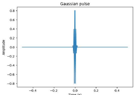
So, overall, this code generates a Gaussian pulse with center frequency 100 Hz, bandwidth 0.5 Hz, and plots it in the time domain over the range of -0.5 to 0.5 seconds.

Example 2: Generating a symmetric Gaussian pulse with a time-bandwidth product of 10

In this example, we will generate a symmetric Gaussian pulse with a time-bandwidth product of 10.

Syntax

import numpy as np
import matplotlib.pyplot as plt
from scipy.signal import gausspulse

t = np.linspace(-10, 10, 500)
fc = 10
bw = 0.5
tpr = 10

p = gausspulse(t, fc=fc, bw=bw, tpr=tpr)

plt.plot(t, p)
plt.title('Gaussian pulse')
plt.xlabel('Time (s)')
plt.ylabel('Amplitude')
plt.show()

The first block imports the necessary libraries and modules, just like in the previous example.

Next line generates a 1D NumPy array t with 500 evenly spaced points between -10 and 10. This array represents the time domain for the pulse.

Following that the lines define the center frequency (fc), bandwidth (bw), and time-bandwidth product (tpr) of the Gaussian pulse.

The time-bandwidth product is a parameter that describes the duration of the pulse in relation to its bandwidth. Specifically, it is the product of the pulse duration (in seconds) and the bandwidth (in Hz). In this case, tpr is set to 10, which means that the pulse has a duration of 1 second (tpr / bw) and a bandwidth of 0.5 Hz.

The line with variable p generates the Gaussian pulse p using the gausspulse function from the Scipy signal module.

The last block of lines plot the generated Gaussian pulse using Matplotlib's plot function. The title, x-label, and y-label are also defined using title, xlabel, and ylabel, respectively. The plot is then displayed using show().

Output

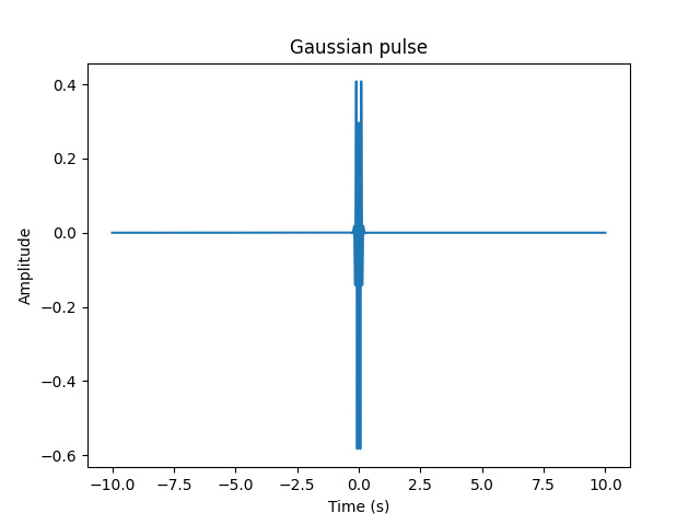
So in the output, this code generates a Gaussian pulse with center frequency 10 Hz, bandwidth 0.5 Hz, and time-bandwidth product 10, and plots it in the time domain over the range of -10 to 10 seconds.

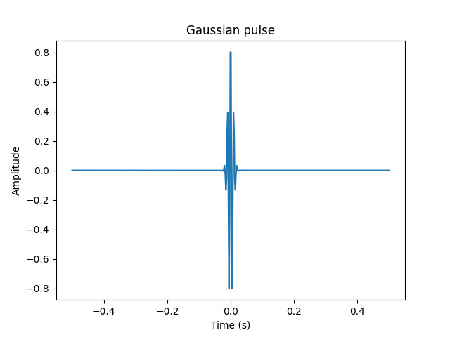
Final Program,Code

# Example 1 code
import numpy as np
import matplotlib.pyplot as plt
from scipy.signal import gausspulse

t = np.linspace(-0.5, 0.5, 500)
fc = 100
bw = 0.5

p = gausspulse(t, fc=fc, bw=bw)

plt.plot(t, p)
plt.title('Gaussian pulse')
plt.xlabel('Time (s)')
plt.ylabel('Amplitude')
plt.show()

# Example 2 code
import numpy as np
import matplotlib.pyplot as plt
from scipy.signal import gausspulse

t = np.linspace(-10, 10, 500)
fc = 10
bw = 0.5
tpr = 10

p = gausspulse(t, fc=fc, bw=bw, tpr=tpr)

plt.plot(t, p)
plt.title('Gaussian pulse')
plt.xlabel('Time (s)')
plt.ylabel('Amplitude')
plt.show()

Output

Conclusion

In this tutorial, we have explored how to generate Gaussian pulses using the scipy.signal.gausspulse function. This function is useful for generating pulses that are widely used in signal processing, particularly in radar, sonar, and communications. The function has several parameters that can be used to control the shape and properties of the pulse, including the time sampling, center frequency, fractional bandwidth, time-bandwidth product, and symmetry. By understanding the properties of Gaussian pulses and how to generate them using the scipy library, you can apply them to various signal processing applications.