Advanced Excel - Slicers

Slicers were introduced in Excel 2010 to filter the data of pivot table. In Excel 2013, you can create Slicers to filter your table data also.

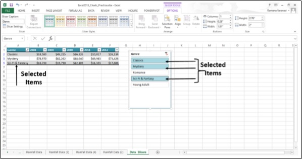
A Slicer is useful because it clearly indicates what data is shown in your table after you filter your data.

Step 1 − Click in the Table. TABLE TOOLS tab appears on the ribbon.

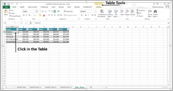
Step 2 − Click on DESIGN. The options for DESIGN appear on the ribbon.

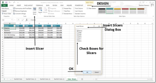
Step 3 − Click on Insert Slicer. A Insert Slicers dialog box appears.

Step 4 − Check the boxes for which you want the slicers. Click on Genre.

Step 5 − Click OK.

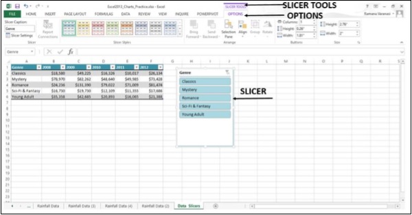
The slicer appears. Slicer tools appear on the ribbon. Clicking the OPTIONS button, provides various Slicer Options.

Step 6 − In the slicer, click the items you want to display in your table. To choose more than one item, hold down CTRL, and then pick the items you want to show.