- Excel - Chart Recommendations
- Advanced Excel - Format Charts
- Advanced Excel - Chart Design
- Advanced Excel - Richer Data Labels
- Advanced Excel - Leader Lines
- Advanced Excel - New Functions
- Fundamental Data Analysis
- Excel - Instant Data Analysis
- Excel - Sorting Data by Color
- Advanced Excel - Slicers
- Advanced Excel - Flash Fill
- Powerful Data Analysis
- Excel - PivotTable Recommendations
- Powerful Data Analysis – 1
- Advanced Excel - Data Model
- Advanced Excel - Power Pivot
- Excel - External Data Connection
- Advanced Excel - Pivot Table Tools
- Powerful Data Analysis – 2
- Advanced Excel - Power View
- Advanced Excel - Visualizations
- Advanced Excel - Pie Charts
- Advanced Excel - Additional Features
- Advanced Excel - Power View Services
- Advanced Excel - Format Reports
- Advanced Excel - Handling Integers
- Other Features
- Advanced Excel - Templates
- Advanced Excel - Inquire
- Advanced Excel - Workbook Analysis
- Advanced Excel - Manage Passwords
- Advanced Excel - File Formats
- Excel - Discontinued Features
- Advanced Excel Useful Resources
- Advanced Excel - Quick Guide
- Advanced Excel - Useful Resources
- Advanced Excel - Discussion
Advanced Excel - Format Reports
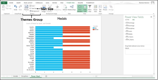
In Excel 2013, Power View has 39 additional themes with more varied chart palettes as well as fonts and background colors. When you change the theme, the new theme applies to all the Power View Views in the Report or Sheets in the Workbook.
You can also change the text size for all of your Report Elements.
You can add Background Images, choose Background Formatting, choose a Theme, change the Font Size for One Visualization, change the Font or Font Size for the whole sheet and Format numbers in a Table, Card, or Matrix.
Step 1 − Click on the Power View tab on the ribbon.
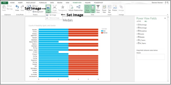
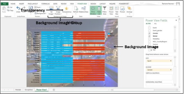
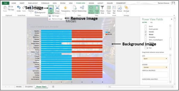
Step 2 − Click on Set Image in the Background Image group.
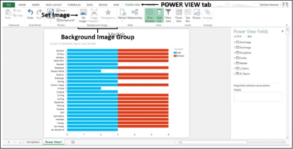
Step 3 − Click on Set Image in the drop-down menu. The File Browser opens.
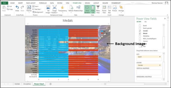
Step 4 − Browse to the Image File you want to use as Background and click open. The image appears as background in the Power View.
Step 5 − Click on Image Position in the Background Image group.
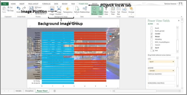
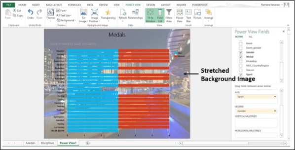
Step 6 − Click on Stretch in the Drop down menu as shown in the image given below.
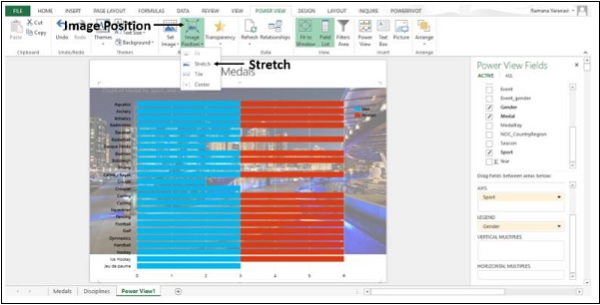
The Image stretches to the full size of Power View.
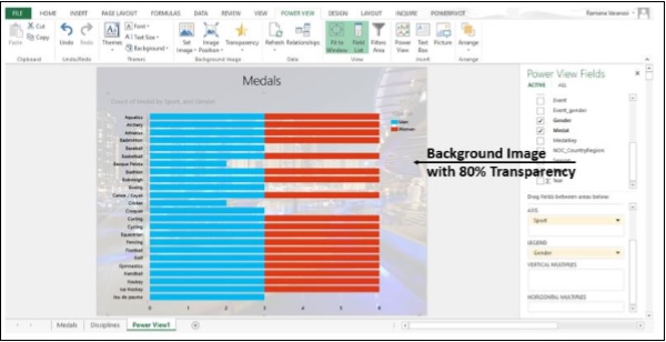
Step 7 − Click on Transparency in the Background Image group.
Step 8 − Click on 80% in the Drop down box.
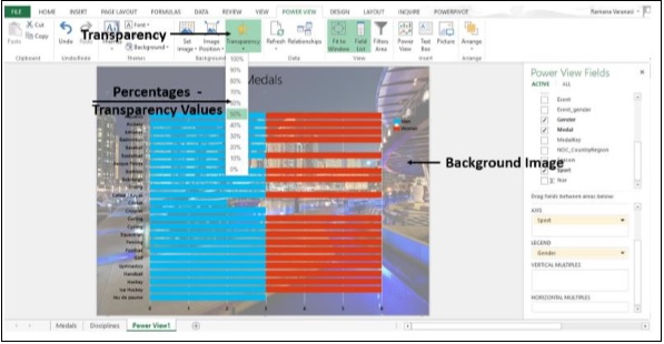
The higher the percentage, the more transparent (less visible) the image.
Instead of images, you can also set different backgrounds to Power View.
Step 9 − Click on Power View tab on the ribbon.
Step 10 − Click on Set Image in the Background Image group.
Step 11 − Click on Remove Image.
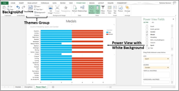
Now, Power View is with White Background.
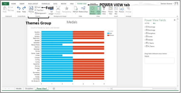
Step 12 − Click on Background in the Themes Group.
You have different backgrounds, from solids to a variety of gradients.
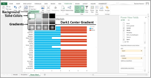
Step 13 − Click on Dark1 Center Gradient.
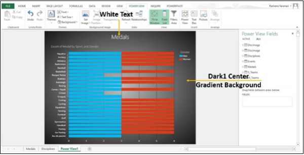
The background changes to Dark1 Center Gradient. As the background is darker, the text turns into white color.
Step 14 − Click on the Power View tab on the ribbon.
Step 15 − Click on Font in the Themes group.
All the available fonts will be displayed in the Drop down list.
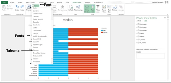
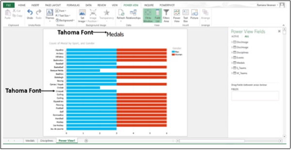
Step 16 − Click on Tahoma. The font of the text changes to Tahoma.
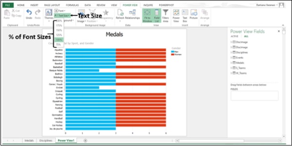
Step 17 − Click on Text Size in the Themes group.
The percentages of the font sizes will be displayed. The default font size 100% is highlighted.
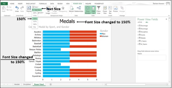
Step 18 − Select 150%. The font size changes from 100% to 150%.
Step 19 − Switch Stacked Bar Chart Visualization to Table Visualization.
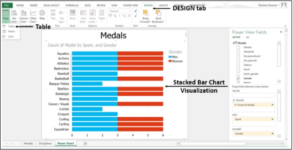
The changed font and font size are retained in the Table Visualization.
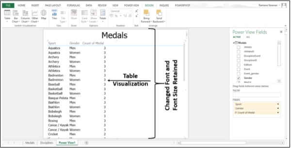
When you change the font in one Visualization, the same font is applied to all visualizations except for the font in a Map Visualization. You cannot have different fonts for different Visualizations. However, you can change the font size for individual visualizations.
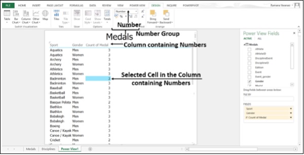
Step 20 − Click on a Cell in the Column containing Numbers.
Step 21 − Click on Number in the Number Group.
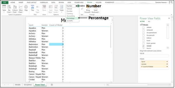
Step 22 − Click on Percentage in the Drop down menu.
The entire column containing the selected cell gets converted to the selected format.
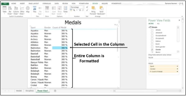
You can format numbers in Card and Matrix Visualizations also.
Hyperlinks
You can add a Hyperlink to a text box in Power View. If Data Model has a field that contains a Hyperlink, add that field to the Power View. It can link to any URL or email address.
This is how you could get the sport images in Tiles in Tiles Visualization in the previous section.
Printing
You can print Power View sheets in Excel 2013. What you print is what you see on the sheet when you send it to the printer. If the sheet or view contains a region with a scroll bar, the printed page contains the part of the region that is visible on the screen. If a sheet or view contains a region with tiles, then whichever tile is selected is the one that prints.
Support for right-to-left languages
Power View in Excel 2013 supports right-to-left languages. Power View takes the setting for default direction from Excel. You can change those settings.
Step 1 − Click on File.
Step 2 − Click on Options. The Excel Options window appears.
Step 3 − By default, the direction has two options Right-to-left and Left-to-right.
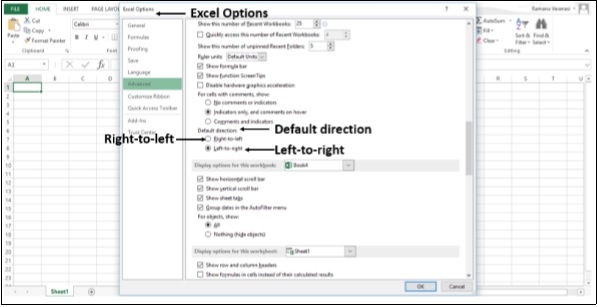
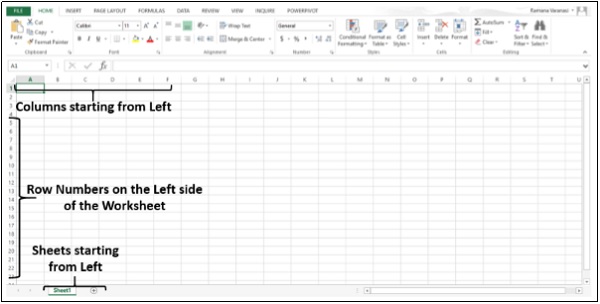
Step 4 − Set the default direction to Left-to-right.
Step 5 − Click OK.
Step 6 − Change the default direction to Right-to-left.
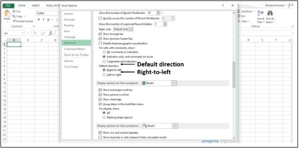
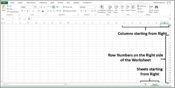
Step 7 − Click OK. You can see that the columns are now starting from the right side of the screen as shown in the image given below.
Microsoft Office supports right-to-left functionality and features for languages that work in a right-to-left or a combined right-to-left, left-to-right environment for entering, editing, and displaying text. In this context, "right-to-left languages" refers to any writing system that is written from right to left and includes languages that require contextual shaping, such as Arabic, and languages that do not. You can change your display to read right-to-left or change individual files so their contents read from right to left.
If your computer does not have a right-to-left language version of Office installed, you will need to install the appropriate language pack. You must also be running a Microsoft Windows operating system that has right-to-left support for example, the Arabic version of Windows Vista Service Pack 2 and enable the keyboard language for the right-to-left language that you want to use.
