Convolution and Correlation

Convolution

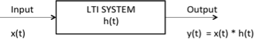
Convolution is a mathematical operation used to express the relation between input and output of an LTI system. It relates input, output and impulse response of an LTI system as

$$ y (t) = x(t) * h(t) $$

Where y (t) = output of LTI

x (t) = input of LTI

h (t) = impulse response of LTI

There are two types of convolutions:

Continuous convolution
Discrete convolution

Continuous Convolution

$ y(t) \,\,= x (t) * h (t) $

$= \int_{-\infty}^{\infty} x(\tau) h (t-\tau)d\tau$

(or)

$= \int_{-\infty}^{\infty} x(t - \tau) h (\tau)d\tau $

Discrete Convolution

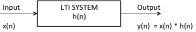
$y(n)\,\,= x (n) * h (n)$

$= \Sigma_{k = - \infty}^{\infty} x(k) h (n-k) $

(or)

$= \Sigma_{k = - \infty}^{\infty} x(n-k) h (k) $

By using convolution we can find zero state response of the system.

Deconvolution

Deconvolution is reverse process to convolution widely used in signal and image processing.

Properties of Convolution

Commutative Property

$ x_1 (t) * x_2 (t) = x_2 (t) * x_1 (t) $

Distributive Property

$ x_1 (t) * [x_2 (t) + x_3 (t) ] = [x_1 (t) * x_2 (t)] + [x_1 (t) * x_3 (t)]$

Associative Property

$x_1 (t) * [x_2 (t) * x_3 (t) ] = [x_1 (t) * x_2 (t)] * x_3 (t) $

Shifting Property

$ x_1 (t) * x_2 (t) = y (t) $

$ x_1 (t) * x_2 (t-t_0) = y (t-t_0) $

$ x_1 (t-t_0) * x_2 (t) = y (t-t_0) $

$ x_1 (t-t_0) * x_2 (t-t_1) = y (t-t_0-t_1) $

Convolution with Impulse

$ x_1 (t) * \delta (t) = x(t) $

$ x_1 (t) * \delta (t- t_0) = x(t-t_0) $

Convolution of Unit Steps

$ u (t) * u (t) = r(t) $

$ u (t-T_1) * u (t-T_2) = r(t-T_1-T_2) $

$ u (n) * u (n) = [n+1] u(n) $

Scaling Property

If $x (t) * h (t) = y (t) $

then $x (a t) * h (a t) = {1 \over |a|} y (a t)$

Differentiation of Output

if $y (t) = x (t) * h (t)$

then $ {dy (t) \over dt} = {dx(t) \over dt} * h (t) $

$ {dy (t) \over dt} = x (t) * {dh(t) \over dt}$

Note:

Convolution of two causal sequences is causal.
Convolution of two anti causal sequences is anti causal.
Convolution of two unequal length rectangles results a trapezium.
Convolution of two equal length rectangles results a triangle.
A function convoluted itself is equal to integration of that function.

Example: You know that $u(t) * u(t) = r(t)$

According to above note, $u(t) * u(t) = \int u(t)dt = \int 1dt = t = r(t)$

Here, you get the result just by integrating $u(t)$.

Limits of Convoluted Signal

If two signals are convoluted then the resulting convoluted signal has following range:

Sum of lower limits < t < sum of upper limits

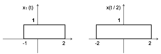
Ex: find the range of convolution of signals given below

Here, we have two rectangles of unequal length to convolute, which results a trapezium.

The range of convoluted signal is:

Sum of lower limits < t < sum of upper limits

$-1+-2 < t < 2+2 $

$-3 < t < 4 $

Hence the result is trapezium with period 7.

Area of Convoluted Signal

The area under convoluted signal is given by $A_y = A_x A_h$

Where A_x = area under input signal

A_h = area under impulse response

A_y = area under output signal

Proof: $y(t) = \int_{-\infty}^{\infty} x(\tau) h (t-\tau)d\tau$

Take integration on both sides

$ \int y(t)dt \,\,\, =\int \int_{-\infty}^{\infty}\, x (\tau) h (t-\tau)d\tau dt $

$ =\int x (\tau) d\tau \int_{-\infty}^{\infty}\, h (t-\tau) dt $

We know that area of any signal is the integration of that signal itself.

$\therefore A_y = A_x\,A_h$

DC Component

DC component of any signal is given by

$\text{DC component}={\text{area of the signal} \over \text{period of the signal}}$

Ex: what is the dc component of the resultant convoluted signal given below?

Here area of x₁(t) = length × breadth = 1 × 3 = 3

area of x₂(t) = length × breadth = 1 × 4 = 4

area of convoluted signal = area of x₁(t) × area of x₂(t)

= 3 × 4 = 12

Duration of the convoluted signal = sum of lower limits < t < sum of upper limits

= -1 + -2 < t < 2+2

= -3 < t < 4

Period=7

$\therefore$ Dc component of the convoluted signal = $\text{area of the signal} \over \text{period of the signal}$

Dc component = ${12 \over 7}$

Discrete Convolution

Let us see how to calculate discrete convolution:

i. To calculate discrete linear convolution:

Convolute two sequences x[n] = {a,b,c} & h[n] = [e,f,g]

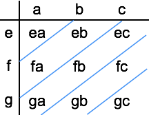
Convoluted output = [ ea, eb+fa, ec+fb+ga, fc+gb, gc]

Note: if any two sequences have m, n number of samples respectively, then the resulting convoluted sequence will have [m+n-1] samples.

Example: Convolute two sequences x[n] = {1,2,3} & h[n] = {-1,2,2}

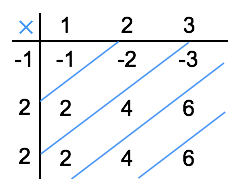
Convoluted output y[n] = [ -1, -2+2, -3+4+2, 6+4, 6]

= [-1, 0, 3, 10, 6]

Here x[n] contains 3 samples and h[n] is also having 3 samples so the resulting sequence having 3+3-1 = 5 samples.

ii. To calculate periodic or circular convolution:

Periodic convolution is valid for discrete Fourier transform. To calculate periodic convolution all the samples must be real. Periodic or circular convolution is also called as fast convolution.

If two sequences of length m, n respectively are convoluted using circular convolution then resulting sequence having max [m,n] samples.

Ex: convolute two sequences x[n] = {1,2,3} & h[n] = {-1,2,2} using circular convolution

Normal Convoluted output y[n] = [ -1, -2+2, -3+4+2, 6+4, 6].

= [-1, 0, 3, 10, 6]

Here x[n] contains 3 samples and h[n] also has 3 samples. Hence the resulting sequence obtained by circular convolution must have max[3,3]= 3 samples.

Now to get periodic convolution result, 1st 3 samples [as the period is 3] of normal convolution is same next two samples are added to 1st samples as shown below:

$\therefore$ Circular convolution result $y[n] = [9\quad 6\quad 3 ]$

Correlation

Correlation is a measure of similarity between two signals. The general formula for correlation is

$$ \int_{-\infty}^{\infty} x_1 (t)x_2 (t-\tau) dt $$

There are two types of correlation:

Auto correlation
Cros correlation

Auto Correlation Function

It is defined as correlation of a signal with itself. Auto correlation function is a measure of similarity between a signal & its time delayed version. It is represented with R($\tau$).

Consider a signals x(t). The auto correlation function of x(t) with its time delayed version is given by

$$ R_{11} (\tau) = R (\tau) = \int_{-\infty}^{\infty} x(t)x(t-\tau) dt \quad \quad \text{[+ve shift]} $$

$$\quad \quad \quad \quad \quad = \int_{-\infty}^{\infty} x(t)x(t + \tau) dt \quad \quad \text{[-ve shift]} $$

Where $\tau$ = searching or scanning or delay parameter.

If the signal is complex then auto correlation function is given by

$$ R_{11} (\tau) = R (\tau) = \int_{-\infty}^{\infty} x(t)x * (t-\tau) dt \quad \quad \text{[+ve shift]} $$

$$\quad \quad \quad \quad \quad = \int_{-\infty}^{\infty} x(t + \tau)x * (t) dt \quad \quad \text{[-ve shift]} $$

Properties of Auto-correlation Function of Energy Signal

Auto correlation exhibits conjugate symmetry i.e. R ($\tau$) = R*(-$\tau$)
Auto correlation function of energy signal at origin i.e. at $\tau$=0 is equal to total energy of that signal, which is given as:

R (0) = E = $ \int_{-\infty}^{\infty}\,|\,x(t)\,|^2\,dt $
Auto correlation function $\infty {1 \over \tau} $,
Auto correlation function is maximum at $\tau$=0 i.e |R ($\tau$) | ≤ R (0) ∀ $\tau$
Auto correlation function and energy spectral densities are Fourier transform pairs. i.e.

$F.T\,[ R (\tau) ] = \Psi(\omega)$

$\Psi(\omega) = \int_{-\infty}^{\infty} R (\tau) e^{-j\omega \tau} d \tau$
$ R (\tau) = x (\tau)* x(-\tau) $

Auto Correlation Function of Power Signals

The auto correlation function of periodic power signal with period T is given by

$$ R (\tau) = \lim_{T \to \infty} {1\over T} \int_{{-T \over 2}}^{{T \over 2}}\, x(t) x* (t-\tau) dt $$

Properties

Auto correlation of power signal exhibits conjugate symmetry i.e. $ R (\tau) = R*(-\tau)$
Auto correlation function of power signal at $\tau = 0$ (at origin)is equal to total power of that signal. i.e.

$R (0)= \rho $
Auto correlation function of power signal $\infty {1 \over \tau}$,
Auto correlation function of power signal is maximum at $\tau$ = 0 i.e.,

$ | R (\tau) | \leq R (0)\, \forall \,\tau$
Auto correlation function and power spectral densities are Fourier transform pairs. i.e.,

$F.T[ R (\tau) ] = s(\omega)$

$s(\omega) = \int_{-\infty}^{\infty} R (\tau) e^{-j\omega \tau} d\tau$
$R (\tau) = x (\tau)* x(-\tau) $

Density Spectrum

Let us see density spectrums:

Energy Density Spectrum

Energy density spectrum can be calculated using the formula:

$$ E = \int_{-\infty}^{\infty} |\,x(f)\,|^2 df $$

Power Density Spectrum

Power density spectrum can be calculated by using the formula:

$$P = \Sigma_{n = -\infty}^{\infty}\, |\,C_n |^2 $$

Cross Correlation Function

Cross correlation is the measure of similarity between two different signals.

Consider two signals x₁(t) and x₂(t). The cross correlation of these two signals $R_{12}(\tau)$ is given by

$$R_{12} (\tau) = \int_{-\infty}^{\infty} x_1 (t)x_2 (t-\tau)\, dt \quad \quad \text{[+ve shift]} $$

$$\quad \quad = \int_{-\infty}^{\infty} x_1 (t+\tau)x_2 (t)\, dt \quad \quad \text{[-ve shift]}$$

If signals are complex then

$$R_{12} (\tau) = \int_{-\infty}^{\infty} x_1 (t)x_2^{*}(t-\tau)\, dt \quad \quad \text{[+ve shift]} $$

$$\quad \quad = \int_{-\infty}^{\infty} x_1 (t+\tau)x_2^{*} (t)\, dt \quad \quad \text{[-ve shift]}$$

$$R_{21} (\tau) = \int_{-\infty}^{\infty} x_2 (t)x_1^{*}(t-\tau)\, dt \quad \quad \text{[+ve shift]} $$

$$\quad \quad = \int_{-\infty}^{\infty} x_2 (t+\tau)x_1^{*} (t)\, dt \quad \quad \text{[-ve shift]}$$

Properties of Cross Correlation Function of Energy and Power Signals

Auto correlation exhibits conjugate symmetry i.e. $R_{12} (\tau) = R^*_{21} (-\tau)$.
Cross correlation is not commutative like convolution i.e.

$$ R_{12} (\tau) \neq R_{21} (-\tau) $$
If R₁₂(0) = 0 means, if $ \int_{-\infty}^{\infty} x_1 (t) x_2^* (t) dt = 0$, then the two signals are said to be orthogonal.

For power signal if $ \lim_{T \to \infty} {1\over T} \int_{{-T \over 2}}^{{T \over 2}}\, x(t) x^* (t)\,dt $ then two signals are said to be orthogonal.
Cross correlation function corresponds to the multiplication of spectrums of one signal to the complex conjugate of spectrum of another signal. i.e.

$$ R_{12} (\tau) \leftarrow \rightarrow X_1(\omega) X_2^*(\omega)$$

This also called as correlation theorem.

Parseval's Theorem

Parseval's theorem for energy signals states that the total energy in a signal can be obtained by the spectrum of the signal as

$ E = {1\over 2 \pi} \int_{-\infty}^{\infty} |X(\omega)|^2 d\omega $

Note: If a signal has energy E then time scaled version of that signal x(at) has energy E/a.