- Home
- Introduction
- Modulation
- Noise
- Analyzing Signals
- Amplitude Modulation
- Sideband Modulation
- VSB Modulation
- Angle Modulation
- Multiplexing
- FM Radio
- Pulse Modulation
- Analog Pulse Modulation
- Digital Modulation
- Modulation Techniques
- Delta Modulation
- Digital Modulation Techniques
- M-ary Encoding
- Information Theory
- Spread Spectrum Modulation
- Optical Fiber Communications
- Satellite Communications
Pulse Modulation
So far, we have discussed about continuous-wave modulation. Now its time for discrete signals. The Pulse modulation techniques, deals with discrete signals. Let us see how to convert a continuous signal into a discrete one. The process called Sampling helps us with this.
Sampling
The process of converting continuous time signals into equivalent discrete time signals, can be termed as Sampling. A certain instant of data is continually sampled in the sampling process.
The following figure indicates a continuous-time signal x(t) and a sampled signal xs(t). When x(t) is multiplied by a periodic impulse train, the sampled signal xs(t) is obtained.
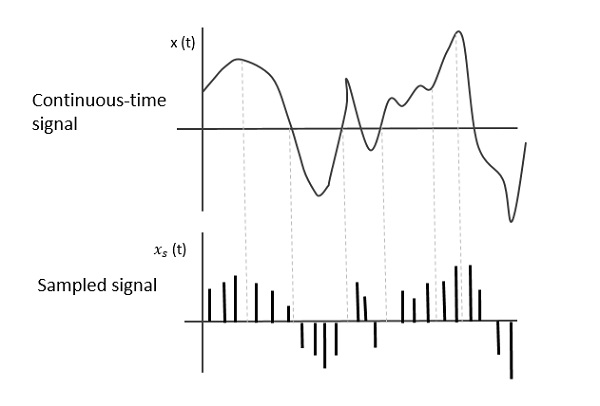
A sampling signal is a periodic train of pulses, having unit amplitude, sampled at equal intervals of time Ts, which is called as the Sampling time. This data is transmitted at the time instants Ts and the carrier signal is transmitted at the remaining time.
Sampling Rate
To discretize the signals, the gap between the samples should be fixed. That gap can be termed as the sampling period Ts.
$$Sampling\:Frequency = \frac{1}{T_s} = f_s$$
Where,
Ts = the sampling time
fs = the sampling frequency or sampling rate
Sampling Theorem
While considering the sampling rate, an important point regarding how much the rate has to be, should be considered. The rate of sampling should be such that the data in the message signal should neither be lost nor it should get over-lapped.
The sampling theorem states that, a signal can be exactly reproduced if it is sampled at the rate fs which is greater than or equal to twice the maximum frequency W.
To put it in simpler words, for the effective reproduction of the original signal, the sampling rate should be twice the highest frequency.
Which means,
$$f_s \geq 2W$$
Where,
fs = the sampling frequency
W is the highest frequency
This rate of sampling is called as Nyquist rate.
The sampling theorem, which is also called as Nyquist theorem, delivers the theory of sufficient sample rate in terms of bandwidth for the class of functions that are bandlimited.
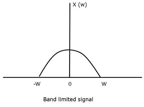
For the continuous-time signal x(t), the band-limited signal in frequency domain, can be represented as shown in the following figure.
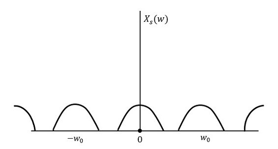
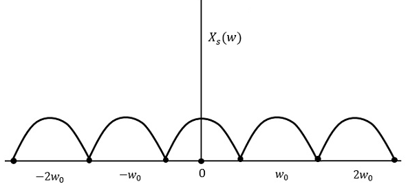
If the signal is sampled above the Nyquist rate, the original signal can be recovered. The following figure explains a signal, if sampled at a higher rate than 2w in the frequency domain.
If the same signal is sampled at a rate less than 2w, then the sampled signal would look like the following figure.
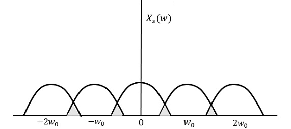
We can observe from the above pattern that the over-lapping of information is done, which leads to mixing up and loss of information. This unwanted phenomenon of over-lapping is called as Aliasing.
Aliasing can be referred to as the phenomenon of a high-frequency component in the spectrum of a signal, taking on the identity of a lower-frequency component in the spectrum of its sampled version.
Hence, the sampling of the signal is chosen to be at the Nyquist rate, as was stated in the sampling theorem. If the sampling rate is equal to twice the highest frequency (2W).
That means,
$$f_s = 2W$$
Where,
fs = the sampling frequency
W is the highest frequency
The result will be as shown in the above figure. The information is replaced without any loss. Hence, this is a good sampling rate.
