- Home
- Introduction
- Linear Programming
- Norm
- Inner Product
- Minima and Maxima
- Convex Set
- Affine Set
- Convex Hull
- Caratheodory Theorem
- Weierstrass Theorem
- Closest Point Theorem
- Fundamental Separation Theorem
- Convex Cones
- Polar Cone
- Conic Combination
- Polyhedral Set
- Extreme point of a convex set
- Direction
- Convex & Concave Function
- Jensen's Inequality
- Differentiable Convex Function
- Sufficient & Necessary Conditions for Global Optima
- Quasiconvex & Quasiconcave functions
- Differentiable Quasiconvex Function
- Strictly Quasiconvex Function
- Strongly Quasiconvex Function
- Pseudoconvex Function
- Convex Programming Problem
- Fritz-John Conditions
- Karush-Kuhn-Tucker Optimality Necessary Conditions
- Algorithms for Convex Problems
Convex Optimization - Linear Programming
Methodology
Linear Programming also called Linear Optimization, is a technique which is used to solve mathematical problems in which the relationships are linear in nature. the basic nature of Linear Programming is to maximize or minimize an objective function with subject to some constraints. The objective function is a linear function which is obtained from the mathematical model of the problem. The constraints are the conditions which are imposed on the model and are also linear.
- From the given question, find the objective function.
- find the constraints.
- Draw the constraints on a graph.
- find the feasible region, which is formed by the intersection of all the constraints.
- find the vertices of the feasible region.
- find the value of the objective function at these vertices.
- The vertice which either maximizes or minimizes the objective function (according to the question) is the answer.
Examples
Step 1 − Maximize $5x+3y$ subject to
$x+y\leq 2$,
$3x+y\leq 3$,
$x\geq 0 \:and \:y\geq 0$
Solution −
The first step is to find the feasible region on a graph.
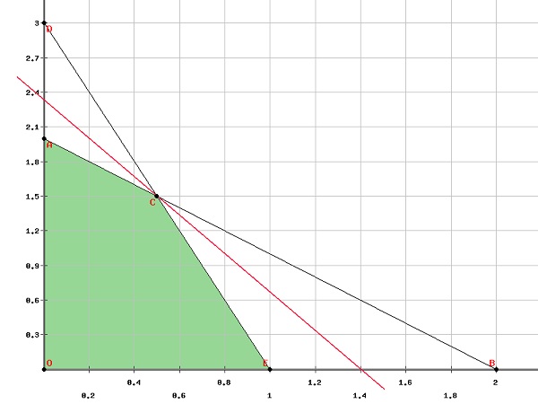
Clearly from the graph, the vertices of the feasible region are
$\left ( 0, 0 \right )\left ( 0, 2 \right )\left ( 1, 0 \right )\left ( \frac{1}{2}, \frac{3}{2} \right )$
Let $f\left ( x, y \right )=5x+3y$
Putting these values in the objective function, we get −
$f\left ( 0, 0 \right )$=0
$f\left ( 0, 2 \right )$=6
$f\left ( 1, 0 \right )$=5
$f\left ( \frac{1}{2}, \frac{3}{2} \right )$=7
Therefore, the function maximizes at $\left ( \frac{1}{2}, \frac{3}{2} \right )$
Step 2 − A watch company produces a digital and a mechanical watch. Long-term projections indicate an expected demand of at least 100 digital and 80 mechanical watches each day. Because of limitations on production capacity, no more than 200 digital and 170 mechanical watches can be made daily. To satisfy a shipping contract, a total of at least 200 watches much be shipped each day.
If each digital watch sold results in a $\$2$ loss, but each mechanical watch produces a $\$5$ profit, how many of each type should be made daily to maximize net profits?
Solution −
Let $x$ be the number of digital watches produced
$y$ be the number of mechanical watches produced
According to the question, at least 100 digital watches are to be made daily and maximaum 200 digital watches can be made.
$\Rightarrow 100 \leq \:x\leq 200$
Similarly, at least 80 mechanical watches are to be made daily and maximum 170 mechanical watches can be made.
$\Rightarrow 80 \leq \:y\leq 170$
Since at least 200 watches are to be produced each day.
$\Rightarrow x +y\leq 200$
Since each digital watch sold results in a $\$2$ loss, but each mechanical watch produces a $\$5$ profit,
Total profit can be calculated as
$Profit =-2x + 5y$
And we have to maximize the profit, Therefore, the question can be formulated as −
Maximize $-2x + 5y$ subject to
$100 \:\leq x\:\leq 200$
$80 \:\leq y\:\leq 170$
$x+y\:\leq 200$
Plotting the above equations in a graph, we get,
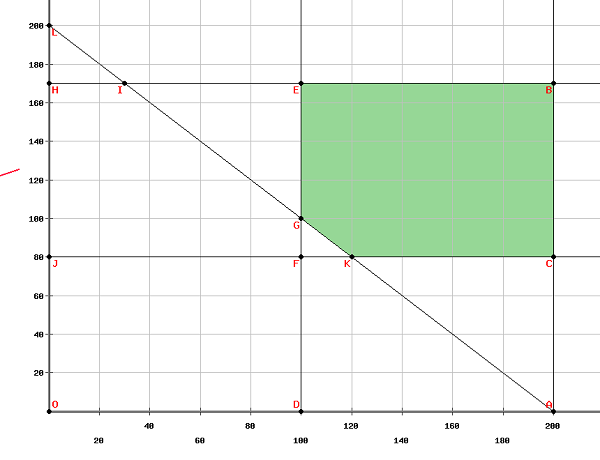
The vertices of the feasible region are
$\left ( 100, 170\right )\left ( 200, 170\right )\left ( 200, 180\right )\left ( 120, 80\right ) and \left ( 100, 100\right )$
The maximum value of the objective function is obtained at $\left ( 100, 170\right )$ Thus, to maximize the net profits, 100 units of digital watches and 170 units of mechanical watches should be produced.