LightGBM - Regression

Quiz

The popular machine−learning method LightGBM (Light Gradient Boosting Machine) is used for regression and classification applications. When it is used for regression, it creates a series of decision trees each trying to minimize a loss function (e.g. mean squared error) by reducing the error from the previous one.

How LightGBM Works for Regression ?

LightGBM's foundation, gradient boosting, creates several decision trees one after the other in an ordered manner. Every tree makes an effort to correct the errors made by previous ones.

Unlike other boosting algorithms, which grow trees level−wise, LightGBM builds trees leaf−wise. This shows that while expanding the model, it optimizes loss reduction (i.e., the leaf that improves the model the most). This provides a deeper and more accurate tree but it needs careful adjustment to avoid overfitting.

To reduce the difference between expected and actual results, LightGBM uses two types of loss functions for regression tasks− mean squared error (MSE) and mean absolute error (MAE).

When to Use LightGBM Regression

Here are some cases when you can use regression using LightGBM −

When a large dataset is given.
When a quick and efficient model is needed.
When your data contains a large number of characteristics (columns) or missing values.

Example of using LightGBM for Regression

Now let's have a look at how to create a LightGBM regression model. These steps will help you understand how each step of the process works.

Step 1 − Install Required Libraries

Before you start make sure you have installed the necessary libraries. Scikit-learn is needed for data manipulation and lightgbm is needed for the LightGBM model.

pip install pandas scikit-learn lightgbm

Step 2 − Load the Data

At first, the dataset is loaded using pandas. This dataset contains health related information including age, gender, BMI, number of children, location, smoking status, and medical bills.

import pandas as pd

# Load the dataset from your local file path
data = pd.read_csv('/My Docs/Python/medical_cost.csv')

# Display the first few rows of the dataset
print(data.head())

Output

This will produce the following result−

   age     sex     bmi  children smoker     region      charges
0   19  female  27.900         0    yes  southwest  16884.92400
1   18    male  33.770         1     no  southeast   1725.55230
2   28    male  33.000         3     no  southeast   4449.46200
3   33    male  22.705         0     no  northwest  21984.47061
4   32    male  28.880         0     no  northwest   3866.85520

Step 3 − Separate Features and Target Variable

The target variable (y) and the features (X) are now being separated. In this case, we want to figure out the 'charges' column using the other features.

# 'charges' is the target column that we want to predict
# All columns except 'charges' are features
X = data.drop('charges', axis=1)  

# The 'charges' column is the target variable
y = data['charges']

Step 4 − Handle Categorical Data

The categorical features in the dataset (gender, smoker, and region) need to be transformed into a numerical format because LightGBM works with numerical data. One-hot encoding is used to convert these category columns into a binary format (0s and 1s).

# Convert categorical variables to numerical 
X = pd.get_dummies(X, drop_first=True)

Here,

pd.get_dummies() is generating additional binary columns for each category.
drop_first=True avoids multicollinearity by eliminating each categorical variable's initial category.

Step 5 − Split the Data

To know the model's performance we will split the data into two sets − a training set means 80% of the data and a testing set means 20% of the data.

train_test split() is used to split the data randomly also maintaining the given proportions (test_size=0.2).
Using the random_state = 42 we will make sure the split can be reproducible.

from sklearn.model_selection import train_test_split

# Split the data into training and test sets
X_train, X_test, y_train, y_test = train_test_split(X, y, test_size=0.2, random_state=42)

Step 6: Initialize the LightGBM Regressor

Now we will initialize the LightGBM model for regression. The LGBMRegressor is the name of the LightGBM implementation created specifically for regression tasks. The LGBMRegressor model is very efficient and flexible, can handle large datasets effectively.

from lightgbm import LGBMRegressor

# Initialize the LightGBM regressor model
model = LGBMRegressor()

Step 7: Train the Model

Next we will train the model with the help of the training data (X_train and y_train). Here the fit() method is used to train the model by finding patterns in the training data and predicting the target variable (charges).

# Train the model on the training data
model.fit(X_train, y_train)

Output

After running the above code we will get the following outcome −

[LightGBM] [Info] Auto-choosing col-wise multi-threading, the overhead of testing was 0.001000 seconds.
You can set `force_col_wise=true` to remove the overhead.
[LightGBM] [Info] Total Bins 319
[LightGBM] [Info] Number of data points in the train set: 1070, number of used features: 8
[LightGBM] [Info] Start training from score 13346.089733

 LGBMRegressori
LGBMRegressor()

Step 8: Make Predictions

After training, we use the model to make predictions for the test set (X_test). The model.predict(X_test) generates predicted values for the test set based on patterns learned from training data.

# Predict on the test set
y_pred = model.predict(X_test)

Step 9: Evaluate the Model

We will measure our model's performance with Mean Squared Error (MSE), a popular regression statistic. The difference between the expected and actual numbers is calculated as the mean squared error, or MSE. Better performance is shown by a lower MSE value.

from sklearn.metrics import mean_squared_error

# Calculate the MSE
mse = mean_squared_error(y_test, y_pred)
print(f'Mean Squared Error: {mse}')

Output

This will generate the below output −

Mean Squared Error: 20557383.0620152

Analyze the MSE number to see how well the model predicts the target variable. If the MSE is high, consider updating the model by adjusting hyperparameters or gathering new data.

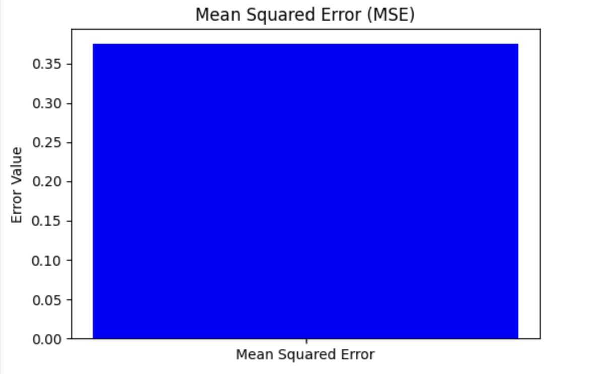
Visualize the Mean Squared Error (MSE)

To see the Mean Squared Error build a bar chart with the MSE value. This provides a clear and visual representation of the problem's magnitude.

Here, you can see how to plot it using matplotlib which is a popular Python library used for plotting −

import matplotlib.pyplot as plt
from sklearn.metrics import mean_squared_error

# Example data (replace these with your actual values)
# Actual values
y_test = [3, -0.5, 2, 7] 

# Predicted values
y_pred = [2.5, 0.0, 2, 8]  

# Calculate the MSE
mse = mean_squared_error(y_test, y_pred)

# Plotting the Mean Squared Error
plt.figure(figsize=(6, 4))
plt.bar(['Mean Squared Error'], [mse], color='blue')
plt.ylabel('Error Value')
plt.title('Mean Squared Error (MSE)')
plt.show()

Output

Here is the result of the above code −

Print Page