LightGBM - Parameter Tuning

Quiz

Optimizing LightGBM's parameters is essential for boosting the model's performance, both in terms of speed and accuracy. This chapter describes in detail how to adjust the most necessary LightGBM parameters.

What is Parameter Tuning ?

Parameter tuning is the process of adjusting a machine learning model's hyperparameters or parameters to maximize performance. In models like LightGBM, hyperparameters that control a model's learning process are leaf count, learning rate, and tree depth.

The parameters are required because −

Boosts Accuracy − On new, untested data, a fine-tuned model generates predicts that are more accurate.
Prevents Overfitting/Underfitting − It ensures that the model is neither too complex nor too simple.
Optimizes Speed − Tuning can reduce training times without affecting performance by using less memory or processor power.

So Let us see how we can tune the parameters of the LightGBM model −

1. Controlling Model Complexity

These are methods for regulating model complexity, balancing underfitting and overfitting by adjusting parameters like as num_leaves and max_depth. Tuning these parameters help us to manage the complexity of the LightGBM model.

num_leaves − It is used to control the number of leaves in each decision tree. More leaves increase model complexity, but too many can lead to overfitting. Set num_leaves less than or equal to 2^(max_depth). For example, if max_depth = 6, set num_leaves <= 64.
min_data_in_leaf − Displays the minimum number of samples, or data points, that a leaf can include. By changing this parameter, you can help the model reduce noise in the data. If the depth is too low, the tree could grow too deeply and become overfit. Values in the hundreds or thousands range are good for large datasets.
max_depth − It is used to limit the depth of the tree. This can help prevent overfitting by limiting the depth to which the trees can grow. So use in combination with num_leaves to control the tree's complexity.

2. Speeding Up the Model

Training speed can be increased without compromising accuracy by using methods like bagging, feature sub-sampling, and max_bin reduction.

Bagging − To speed up training, use a subset of the data in each cycle. By setting the parameters.The percentage of data to be used in each iteration is given by the variable bagging_fraction. The bagging_freq returns the number of bagging iterations per frequency. Two suitable settings to set are bagging_fraction = 0.8 and bagging_freq = 5 to accelerate the model without significantly affecting accuracy.
Feature Sub-sampling − Randomly selects a subset of features to train at each iteration. Use the parameters like feature_fraction. This parameter controls the fraction of features to be used for training. For best practice set feature_fraction = 0.8 to reduce training time.
max_bin − This parameter controls the number of bins used for continuous features. So the best practice is that the max_bin can be decreased to speed up the model and consume less memory, but accuracy can be compromised.
save_binary − Binary data is stored in order to allow faster loading in successive runs. So it is advised to use save_binary=True when running the model repeatedly on the same dataset.

3. Improving Accuracy

Using larger datasets, lower learning rates, and advanced techniques like Dart can improve the model's accuracy, but can come at the cost of longer training durations.

learning_rate and num_iterations − The number of steps and quantity of model modifications made at each iteration are controlled by the parameters learning_rate and num_iterations. Using a smaller learning_rate (like 0.01) and a greater num_iterations (like 1000+) is the best option.
num_leaves − Increased num_leaves makes the model more complex. This may increase accuracy, but if used incorrectly, it may also lead to overfitting. So the best practice is to increase num_leaves if you have enough data, but make sure to combine it with regularization techniques to avoid overfitting.
Training with Bigger Data − More data usually leads to higher accuracy because the model can pick up on a larger range of patterns. So the best practice is to improve the model's ability to generalize, use as much data as possible if overfitting is an issue.
Dart (Dropouts meet Multiple Additive Regression Trees) − This particular version of the gradient boosting technique increases the model's accuracy by randomly deleting trees during training. Therefore, the best practice is to use boosting_type='dart' for issues where you see overfitting or if you are looking for an extra accuracy.
Using Categorical Features − By removing the need to convert categorical features into dummy variables, LightGBM can handle them directly, potentially increasing performance. Therefore, it is better to improve model accuracy by using the categorical_feature option to identify which attributes are categorical.

4. Handling Overfitting

This section explains how subsampling techniques, tree depth restrictions, and regularization are used to prevent the model from overfitting the training set.

max_bin − Using a smaller max_bin can reduce overfitting because it limits the amount of detail in feature binning.
num_leaves − To prevent the training set from being overfit and the model from growing too complicated, decrease the number of leaves in the model.
min_data_in_leaf and min_sum_hessian_in_leaf − These settings help prevent the tree from going too deep by ensuring that each leaf contains a minimum sum of the second derivative (min_sum_hessian_in_leaf) and a minimum amount of data points (min_data_in_leaf). Increase the min_data_in_leaf and min_sum_hessian_in_leaf to avoid overfitting, particularly for small datasets.
Bagging and Feature Sub-sampling − Use feature sub-sampling (feature_fraction) and bagging (bagging_fraction and bagging_freq) to increase unpredictability in the model and reduce overfitting.
Regularization − Defining parameters like lambda_l1 which is L1 regularization, commonly referred to as Lasso, to reduce the complexity of the model. And lambda_l2 is used to reduce overfitting with ridge-based L2 regularization. The minimal gain required to split a tree node is indicated by the variable min_gain_to_split. Try increasing lambda_l1 and lambda_l2 to add regularization to the model, and adjust min_gain_to_split to control how easily the model creates new branches.
max_depth − Set a reasonable max_depth to limit the depth of the trees and avoid overfitting, especially on smaller datasets.

Example of Parameter Tuning in Python

Here is the small example for performing LightGBM parameter tuning in Python −

# Import necessary libraries
import pandas as pd
import numpy as np
import matplotlib.pyplot as plt
import seaborn as sns

from sklearn.model_selection import train_test_split, RandomizedSearchCV
import lightgbm as lgb
from sklearn.metrics import accuracy_score, classification_report, confusion_matrix

sns.set(style="whitegrid", color_codes=True, font_scale=1.3)

import warnings
warnings.filterwarnings('ignore')

# Load dataset
data = pd.read_csv('/Python/breast_cancer_data.csv')
data.head()

# 1. Preprocessing
# Drop unnecessary columns
data = data.drop(columns=['id', 'Unnamed: 32'])

# Convert 'diagnosis' column to numerical (0: Benign, 1: Malignant)
data['diagnosis'] = data['diagnosis'].map({'B': 0, 'M': 1})

# Split the data into features (X) and target (y)
X = data.drop(columns=['diagnosis'])
y = data['diagnosis']

# Clean column names to avoid LightGBM error
X.columns = X.columns.str.replace('[^A-Za-z0-9_]+', '', regex=True)

# Train-test split
X_train, X_test, y_train, y_test = train_test_split(X, y, test_size=0.2, random_state=42)

# 2. Define parameter grid for tuning
param_grid = {
    'learning_rate': [0.01, 0.05, 0.1],
    'num_leaves': [20, 31, 40],
    'max_depth': [-1, 10, 20],
    'feature_fraction': [0.6, 0.8, 1.0],
    'bagging_fraction': [0.6, 0.8, 1.0],
    'bagging_freq': [0, 5, 10],
    'lambda_l1': [0, 1, 5],
    'lambda_l2': [0, 1, 5]
}

# 3. Set up the LightGBM model
lgb_estimator = lgb.LGBMClassifier(objective='binary', metric='binary_logloss')

# 4. Perform Randomized Search for parameter tuning
random_search = RandomizedSearchCV(estimator=lgb_estimator, param_distributions=param_grid, 
                                   n_iter=50, scoring='accuracy', cv=5, verbose=1, random_state=42)

# 5. Fit the model
random_search.fit(X_train, y_train)

# 6. Get the best parameters
print("Best Parameters:", random_search.best_params_)

# 7. Predict and evaluate the model
y_pred = random_search.predict(X_test)
accuracy = accuracy_score(y_test, y_pred)
print(f"Accuracy: {accuracy * 100:.2f}%")

# Confusion Matrix
conf_matrix = confusion_matrix(y_test, y_pred)
print("Confusion Matrix:")
print(conf_matrix)

# Classification report
print("Classification Report:")
print(classification_report(y_test, y_pred))

# Optional: Plot Confusion Matrix for visualization
plt.figure(figsize=(8,6))
sns.heatmap(conf_matrix, annot=True, fmt='d', cmap='Blues', xticklabels=['Benign', 'Malignant'], yticklabels=['Benign', 'Malignant'])
plt.xlabel('Predicted')
plt.ylabel('Actual')
plt.title('Confusion Matrix')
plt.show()

Output

Here is the output of the above parameter tuning of LightGBM model −

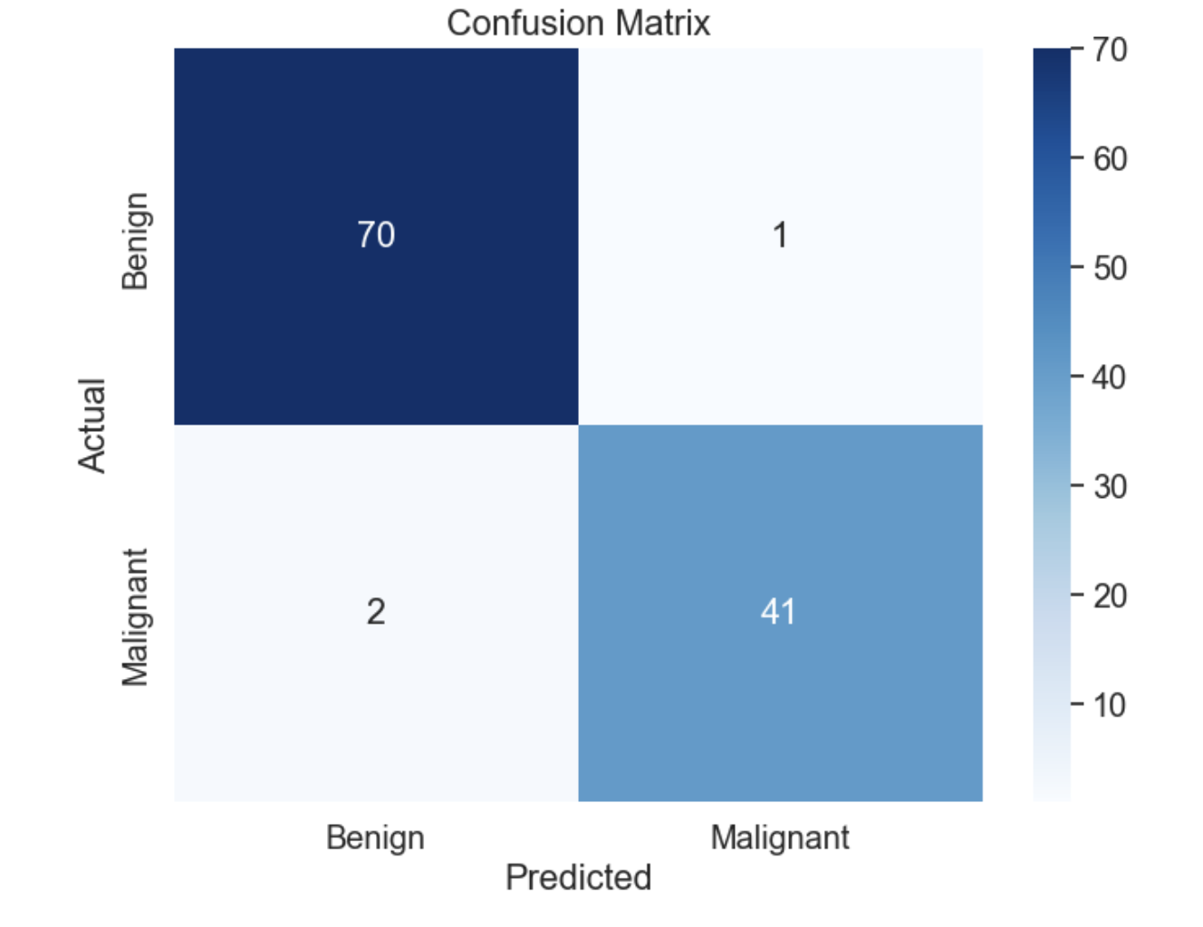
Accuracy: 97.37%
Confusion Matrix:
[[70  1]
 [ 2 41]]
Classification Report:
              precision    recall  f1-score   support

           0       0.97      0.99      0.98        71
           1       0.98      0.95      0.96        43

    accuracy                           0.97       114
   macro avg       0.97      0.97      0.97       114
weighted avg       0.97      0.97      0.97       114

The confusion matrix is as follows −

Summary

LightGBM parameters need to be tuned in order to maximize model performance and training speed. Finding a balance between speed, precision, complexity, and overfitting prevention is key. By carefully adjusting parameters like num_leaves, min_data_in_leaf, bagging_fraction, and max_depth, you can build a model that performs well on both training and unseen data. Here, L1 and L2 regularization procedures can help further prevent overfitting and enhance the model's generalization.

Print Page