LightGBM - Quick Guide

Quiz

LightGBM - Overview

LightGBM is a very effective and fast tool for building machine learning models. It uses advanced methods to speed up and scale up the training process, like efficient data processing and the development of trees using the leaf-wise growth strategy. As a result, it is a great option for managing complex models and large datasets.

LightGBM reduces memory usage and training time using technologies like GOSS (Gradient-based One-Side Sampling) and EFB (Exclusive Feature Bundling). It is also much quicker than traditional boosting methods because of GPU acceleration and parallel processing.

How LightGBM Works?

LightGBM uses a specific type of decision tree called "leaf−wise" tree growth. Unlike conventional trees, which grow level by level, trees with LightGBM are grown by growing the leaf that has the best ability to reduce mistake. Generally the result of this strategy is smaller and more precise trees.

Key Features

Here are some common features of the LightGBM −

High Efficiency and Speed: LightGBM's architecture is very fast. Because it uses "histogram-based algorithms" to form trees quickly, it is much faster than other boosting algorithms.
Decreased Memory Usage − LightGBM uses less memory by keeping only the data needed to build trees. So it is suitable for large datasets.
Support for Large Datasets: LightGBM's ability to handle large datasets and high-dimensional, or full of features, data makes it perfect for big data applications.
Accuracy: LightGBM is well known for its high level of accuracy. The model frequently performs very well on a number of machine learning tasks, like value prediction and data classification.
Handling of Missing Data: LightGBM can handle missing data automatically, reducing the need for further pre-processing steps. This is the built-in feature of LightGBM.

Advantages of LightGBM

Here are the main advantages of using LightGBM −

Faster training speed and higher efficiency: Light GBM is a histogram-based technique, which buckets ongoing feature values into discrete bins, resulting in a faster training phase.
Lower memory consumption: Transforms continuous values into discrete bins, which leads to less memory usage.
Improved accuracy: It generates much more complex trees by using a leaf-wise split strategy rather than a level-wise approach, which is the primary element in achieving higher precision.
Compatibility with huge Datasets: It performs equally well with huge datasets while taking significantly less training time than XGBoost.

Disadvantages of LightGBM

Below are some drawbacks of LightGBM you should consider while using it −

Over-fitting: Light GBM divides the tree leaf-wise, which could result to over-fitting because it produces more complicated trees.
Compatibility with Datasets: Light GBM is vulnerable to over-fitting and so can easily over-fit small data sets.
Resource intensive: While it is efficient, training very big models can still be computationally and memory-intensive.
Data Sensitivity: LightGBM might be affected by the data pretreatment method used so it needs careful feature scaling and normalization.

When to Use LightGBM

LightGBM is one of the best machine learning framework. Here are some of the situations in which you can use LightGBM −

Large datasets: LightGBM performs well on big data.
High−dimensional data: When you have many features.
Fast training: If you need to train models quickly.

Use Cases for LightGBM

Here are some use cases where you can use LightGBM −

Predicting house prices
Credit risk analysis
Customer behavior prediction
Ranking problems like search engine results

LightGBM is an efficient and fast technique for many machine learning applications, particularly if dealing with large datasets require high accuracy. Its speed and efficiency make it popular across a wide range of industries.

Microsoft created LightGBM (Light Gradient Boosting Machine), which was officially released as an open source project in 2017. Below is a brief history of its growth.

LightGBM History

Here are the key points in LightGBM history −

Microsoft Research developed LightGBM in 2016 as part of their mission to provide faster and more efficient machine learning tools.
In January 2017, Microsoft released LightGBM as an open-source library on GitHub. The move helped in its growing popularity in the data science community. The upgrade included support for Python, R, and C++, allowing it to be used in a variety of programming environments.
LightGBM introduced important innovations like the leaf−wise growth method for deeper, more accurate trees, GOSS for faster training by selecting critical data points, and EFB for memory savings by combining rarely used features. It also uses a histogram-based technique to speed up training and reduce the use of memory.
LightGBM was widely adopted by the data science community in 2017-2018 because of its speed, accuracy, and efficiency. It became popular in a variety of data science competitions, including those on Kaggle, where it consistently outperformed competing boosting algorithms.
Between 2018 and 2020, LightGBM developers added GPU acceleration support, which improved its speed and made it the preferred choice for large dataset training.
LightGBM's improved handling of categorical features, increased documentation, and community contributions all contributed to its continued competitiveness and popularity.
From 2021 to the present, LightGBM has been continuously developed and maintained, with regular updates to improve performance, introduce new features, and ensure compatibility with the most latest machine learning frameworks.

LightGBM - Architecture

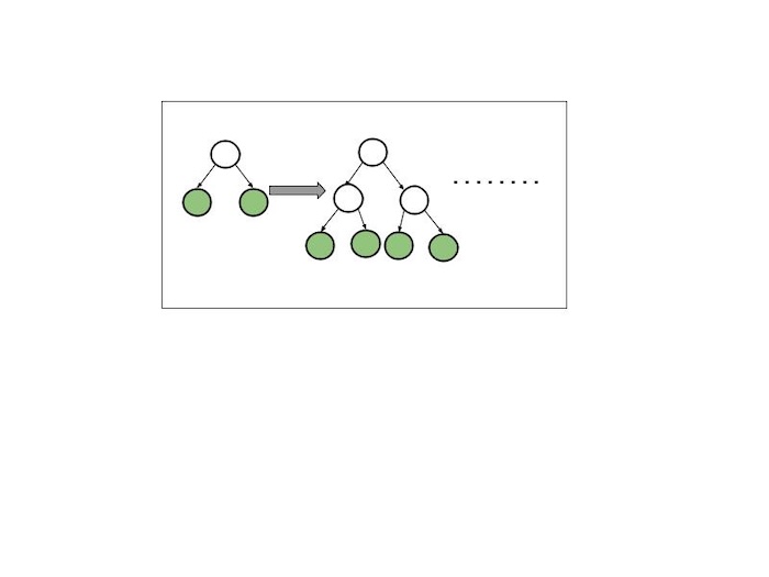
LightGBM divides the tree leaf−wise, whereas other boosting algorithms build it level−wise. It chooses the leaf to split that it believes will result in the largest decrease in loss function. leaf−wise generates splits based on their contribution to the global loss rather than the loss over a specific branch, therefore it sometimes learns lower-error trees "faster" than level−wise.

The diagram below shows the split order of a hypothetical binary leaf−wise tree to a hypothetical binary level−wise tree. It is interesting that the leaf−wise tree can have multiple orderings, whereas the level−wise tree always has the same order.

Leaf−wise Tree Growth

A leaf-wise tree grows by adding branches to the leaf (the end of a branch) that can remove the majority of errors. Consider it similar to developing a tree in a way that focuses on the areas where the model makes the most errors, adding branches just as needed.

This approach makes the tree deeper and more specific in the most important sections, which generally produces a more accurate model, but it can also result in a more complex tree.

Level−wise Tree Growth

A level−wise tree grows by spreading evenly new branches (leaves) over all levels. Consider a tree that grows one layer of branches at a time. It starts by adding branches at level 1, then progresses to level 2, and so on.

This maintains and reduces the tree, but it may not always be the best option because it does not focus on areas which need more detail.

Key Components of LightGBM Architecture

The architecture of LightGBM was created to optimize performance, memory efficiency, and model consistency. Here is a quick overview −

Leaf-Wise Tree Growth: LightGBM grows trees by extending the most important sections first, resulting in deeper, more accurate trees with overall trees.
Histogram-Based Learning: It speeds up training by categorizing data into bins (buckets), which reduce the time and memory needed to find the best splits.
Gradient-based One-Side Sampling (GOSS): GOSS chooses only the most important data points to speed up training while maintaining accuracy.
Exclusive Feature Bundling (EFB): EFB combines rarely seen features to save memory and speed up computations which makes it useful for data with a large number of features.
Parallel and GPU Processing: LightGBM can train models faster by using many CPU cores or GPUs, mainly for large datasets.

LightGBM's design uses leaf-wise tree growth, histogram-based learning, GOSS, and EFB methods to maximize performance and memory usage while maintaining high accuracy. Its parallel and GPU processing power make it perfect for efficiently completing large-scale machine learning tasks.

LightGBM - Installation and Setup

LightGBM is a popular package for machine learning, mainly for gradient boosting. It is fast and efficient, and it is commonly used for Python model development.

LightGBM installations involve setting up the LightGBM gradient boosting framework on a local workstation or server. This usually involves installing necessary dependencies like compilers and CMake, copying the LightGBM repository from GitHub, building the framework with CMake, and installing the Python package using pip.

Proper installation enables users to take advantage of LightGBM's efficient algorithms and functionality for machine learning jobs.

LightGBM can be installed on a number of operating systems, including Windows, macOS, and Linux. Installation steps may vary depending on your operating system. Here's a simple guide for all operating systems −

Installation on Windows

You have three options for installing LightGBM on Windows-Visual Studio, CMake with Visual Studio Build Tools, and CMake with MinGW. Below are the simplified steps for each method −

Using Visual Studio (GUI)

Here are the steps to install LightGBM using Visual Studio −

Install Visual Studio: First you need to download and install Visual Studio in your system.
Download LightGBM: Go to the LightGBM GitHub repository download the zip archive and unzip it.
Open LightGBM in Visual Studio: Navigate to the LightGBM-master/windows folder and open the LightGBM.sln file in Visual Studio. After that choose the "Release" configuration.
Build LightGBM: Click on BUILD &rarrow; Build Solution. If you see errors about the Platform Tool-set so go to PROJECT &rarrow; Properties &rarrow; Configuration Properties &rarrow; General and select the correct tool-set for your machine.
Find the Executable: The .exe file will be located in the LightGBM-master/windows/x64/Release folder.

Using Python Package (pip)

This is the easiest way if you are using Python. So open command prompt in your system and run pip command −

pip install lightgbm

This command will automatically download and install the LightGBM package in your windows system.

Using Anaconda

If you have Anaconda installed then you can use the conda package manager. So open Anaconda prompt or just search for "Anaconda Prompt" in the start menu. And run conda command −

conda install -c conda-forge lightgbm

This will automatically install LightGBM package from the conda−forge channel.

Installation on Linux

LightGBM can be installed on Linux using a number of methods as per your system and preferences. There are three common methods −

Using CMake

Here are the steps to install using CMake in Linux −

Install Required Dependencies: Open a terminal and install the required packages.

sudo apt-get update
sudo apt-get install 
       -y build-essential git cmake libboost-all-dev

Now, you have to clone the LightGBM repository −

git clone --recursive https://github.com/microsoft/LightGBM
cd LightGBM

Build LightGBM: Build LightGBM using the following commands −
```
mkdir build
cd build
cmake ..
make -j4
```
Verify Installation: The LightGBM executable (lightgbm) will be available in the LightGBM/build directory.

Using Python Package (pip)

Here are the steps to install using Python Package (pip) in Linux −

Install Python and pip: Make sure you have Python (3.5 or higher) and pip installed. Install them as needed.
```
sudo apt-get update
sudo apt-get install -y python3 python3-pip
```
Install LightGBM Using pip: Now run the below command to install LightGBM directly using pip.
```
pip install lightgbm
```
Verify Installation: Check that the LightGBM is installed by executing the below command −
```
python3 -c "import lightgbm; print(lightgbm.__version__)"
```

Installation on MacOS

Here are the steps to install LightGBM on macOS −

Install Using Homebrew

Here are the steps to install using Homebrew in MacOS −

Open the terminal using command + space and type "Terminal" then press Enter.
Run the below command in the terminal −
```
brew install lightgbm
```

On successful installation this will generates a message similar to the following −

Install LightGBM Using pip

Here are the steps to install using pip in MacOS −

Install the latest version of Python3 in your MacOS.
Now you have to check that pip3 and python3 are installed properly or not. Use the below commands −
```
python3 --version
pip3 --version
```
Then you can upgrade your pip to prevent any future errors while installation process.
```
pip3 install --upgrade pip
```
Now use the below command to install LightGBM in your macOS with the help of pip3.
```
pip3 install lightgbm
```

On successful installation this will generates a message similar to the following −

Build from GitHub

Here are the steps to install using Homebrew in MacOS −

Install CMake by running this command in the terminal −
```
brew install cmake
```
Install OpenMP by running the below command −
```
brew install libomp
```

Now clone the LightGBM repository of github using the below command −

git clone --recursive https://github.com/microsoft/LightGBM
cd LightGBM

Now you need to build LightGBM using the below commands −
```
mkdir build
cd build
cmake ..
make -j4
```

LightGBM is a fast and efficient machine learning package for gradient boosting. Before installing it, the necessary dependencies and tools must be set up. You can then use tools like Visual Studio, CMake, or pip to build and install the package, based on whether you are running Windows, Linux, or macOS.

LightGBM - Core Parameters

These are the main settings or choices that can be changed when using a machine learning model like LightGBM. They control how the model learns from the data, which has an important impact on the model's accuracy and performance.

Using key parameters, the LightGBM model can be customized for your specific data, task, and limitations. By changing these parameters, you can optimize the model's efficiency, speed, and generalization ability.

Why Core Parameters Are Used

Core parameters in LightGBM help you to −

Control Model Complexity: Limit tree size and depth to avoid making the model too simple (missing patterns) or too complex (fitting noise).
Improve Accuracy: Change the model's learning process, like how fast it should learn, to quickly discover the best option.
Prevent Over fitting: Use limitations or penalties to keep the model from learning the noise in the data instead of the underlying patterns.
Speed up training: To speed up training by deciding how much data and how many features to use in each stage.
Fit Different Tasks: Choose the best settings for your specific problem, like regression or classification, and properly monitor performance.

Core Parameters in LightGBM

Here we will focus on the core LightGBM parameters that control the model's behavior −

1. boosting_type (default = 'gbdt')

This parameter controls the boosting technique used in the training process. Options are as follows −

'gbdt' (Gradient Boosting Decision Tree): The default method, called "gradient boosting decision tree," or "gbdt," builds decision trees one after the other using gradient boosting.
'dart' (Dropouts meet Multiple Additive Regression Trees): During training, some trees are randomly eliminated to prevent over-fitting.
'goss' (Gradient-based One-Side Sampling): Significant data points with larger gradients are selected to speed up training.
'rf' (Random Forest): The Random Forest, known as "rf," creates trees independently and aggregates its predictions.

2. objective

Creates the loss function or objective function that LightGBM will try to optimize.

'regression': A technique used to predict continuous variables, such house values.
'binary': Use "binary" for jobs involving binary categorization (for example, yes/no, spam/ham).
'multi-class': To refer to problems involving multi-class categorization, use "multi-class."

3. metric

This parameter offers the evaluation metric that will be used to evaluate the model's performance.

'binary_logloss': The logarithmic loss for binary classification.
'auc': Area under the ROC Curve, mainly used in classification tasks.
'rmse': Refers to the Root Mean Squared Error in regression situations.

4. learning_rate (default = 0.1)

This core parameter controls the step size at each iteration while moving towards a minimum of the loss function.

Lower values (like 0.01) denote a slower learning rate but higher accuracy.
Higher numbers (e.g., 0.1) may allow for faster learning, but there is a risk of missing the optimal response.

5. num_iterations (default = 100)

It is mainly used to set the number of boosting iterations the model should run. Higher values mean more boosting rounds and better learning but it can increase training time.

6. num_leaves (default = 31)

It is used to determine the complexity of each tree.

Higher values provide more complex trees, but may lead to over-fitting.
Lower values simplify trees, reducing the possibility of over-fitting.

7. max_depth (default = -1)

It is mainly used to limit the maximum depth of the tree. And if it is set to -1 means there is no limit.

Lower values (such as 3 or 5) reduce the depth, reducing the model.
Higher numbers allow for deeper trees, which can detect more complex patterns but may over-fit.

8. min_data_in_leaf (default = 20)

It is the minimum number of data points required in a leaf.

Higher numbers lower the possibility of over-fitting by making sure that each leaf has enough data points.
Lower values can improve model flexibility while increasing the danger of over-fitting.

9. feature_fraction (default = 1.0)

It is used to control how many features are used to train each tree.

A score of 1.0 shows complete use of all features.
Values less than 1.0 randomly select a set of subsets, hence preventing over-fitting.

10. bagging_fraction (default = 1.0)

Determines the portion of data points used for training in each iteration.

A value of 1.0 represents all data points.
Lower values contain a random subset, which increases randomness and helps to prevent over-fitting.

11. bagging_freq (default = 0)

Determines the frequency of bagging. If set to a positive value, bagging is enabled, and data is chosen at random per bagging_freq cycle.

12. lambda_l1 & lambda_l2 (default = 0.0)

It controls both L1 and L2 regularization separately. Higher values add regularization to the model, preventing over-fitting by penalizing large values.

13. min_gain_to_split (default = 0.0)

It is the minimal gain needed for creating another division on a leaf node. Higher values create the model more conservative, which prevents over-fitting.

Implementing LightGBM using Core Parameters

Let's use LightGBM to build a model using these core parameters for the Breast Cancer dataset −

Installing LightGBM

First run the below command to install LightGBM in your system −

pip install lightgbm

Importing Libraries and Load Data

After installing the package we will import the required libraries and load the data −

import lightgbm as lgb
from sklearn.datasets import load_breast_cancer
from sklearn.model_selection import train_test_split
from sklearn.metrics import accuracy_score

# Load dataset
data = load_breast_cancer()
X, y = data.data, data.target

# Split data into training and testing sets
X_train, X_test, y_train, y_test = train_test_split(X, y, test_size=0.2, random_state=42)

Defining Core Parameters

Now let us define the core parameters for our model −

# Define LightGBM parameters
params = {
   'boosting_type': 'gbdt',
   'objective': 'binary',
   'metric': 'binary_logloss',
   'num_leaves': 31,
   'learning_rate': 0.05,
   'num_iterations': 100,
   'max_depth': 5,
   'feature_fraction': 0.8,
   'bagging_fraction': 0.8,
   'bagging_freq': 5,
   'lambda_l1': 0.1,
   'lambda_l2': 0.1,
   'min_gain_to_split': 0.01
}

Preparing Data for LightGBM

In this stage we are required to prepare the data for Light Gradient Boosting Machine.

# Prepare data for LightGBM
train_data = lgb.Dataset(X_train, label=y_train)

Training the Model

Now train the model using the prepared dataset −

# Train the LightGBM model
model = lgb.train(params, train_data)

Making Predictions and Evaluating the Model

Now you have to use the trained model to make predictions and evaluate its accuracy −

# Make predictions
y_pred = model.predict(X_test)
y_pred_binary = [1 if pred > 0.5 else 0 for pred in y_pred]

# Evaluate model accuracy
accuracy = accuracy_score(y_test, y_pred_binary)
print(f"Accuracy is as follows: {accuracy}")

This will lead to the following outcome:

Accuracy is as follows: 0.9737

LightGBM - Boosting Algorithms

Before we look at the various boosting algorithms in LightGBM, let us explain what a boosting algorithm is. Boosting is an effective machine learning approach that improves model accuracy. It works by combining multiple weak models (basic models that do not perform well on their own) to create an improved model that can make better predictions.

LightGBM is a popular framework for boosting. It includes a variety of methods for creating powerful predictive models.

LightGBM Boosting Algorithms

LightGBM supports a wide range of boosting techniques. Each has its own method for creating models and making predictions. Here is a list of the main boosting algorithms used in LightGBM −

Gradient Boosting Decision Tree (GBDT)
Random Forest (RF)
DART (Dropouts And Multiple Additive Regression Trees)
Gradient Based One-Side Sampling (GOSS)

Let us go into each of these algorithms −

Gradient Boosting Decision Tree (GBDT)

GBDT is the default and most commonly used algorithm in LightGBM. Here's how it works −

How it works?

GBDT builds a model in stages, with each stage looking for correct errors from the previous level. It uses decision trees to make predictions. A decision tree is similar to a flowchart in that it helps you make decisions based on certain criteria.

GBDT is incredibly powerful and accurate. It is widely used for a range of tasks, like classification and regression.

For example - In a GBDT model the first tree can predict whether a person will buy a product or not. The second tree will learn from the earlier tree's problems and try to solve them, and the cycle will continue.

Advantages of GBDT

Here are the benefits of GBDT algorithm −

High accuracy.
Can handle both numerical and categorical data.
Works well with large datasets.

Random Forest (RF)

Random Forest is another boosting approach that can be used with LightGBM. It is a bit different than GBDT.

How it Works?

Random Forest builds many decision trees, each based on a different random sample of data. It then combines all of the trees to get the final prediction. The goal is to minimize over-fitting, which happens when a model performs well on training data but poorly on new, unlabeled data.

Random Forest is useful for creating a model that is more stable and less vulnerable to errors on new data.

Think about the forest of many trees, with each tree representing a unique decision path. The final choice depends on the majority vote of all the trees.

Advantages of Random Forests

Here are the benefits of Random Forests algorithm −

Handles large datasets with high dimensionality (many features).
Less likely to over-fit than a single decision tree.
Good performance in classification and regression challenges.

DART (Dropouts meet Multiple Additive Regression Trees)

DART is an improved version of GBDT with a unique change. Let us see how it works −

How it Works?

DART is like GBDT but adds the concept of "dropouts." Dropouts are random removals from the model's trees during training. This reduces the model's dependency on a single tree, resulting in it being more robust and resistant to over-fitting.

If your GBDT model is over-fitting, look into upgrading to DART. It adds regularization into the model, which enhances its performance on new data.

Suppose you are playing a game in which you have to answer questions, some of which are randomly eliminated. It allows you to pay more attention to the remaining questions, which leads to a better overall performance.

Advantages of DART

Here are the benefits of DART algorithm −

Reduces over-fitting by using the dropout method.
Maintains high accuracy while boosting generalization.

GOSS (Gradient-based One-Side Sampling)

GOSS is a boosting algorithm created for speed and efficiency. GOSS shows the most significant data points to speed up training. It accomplishes this by selecting only the data points with the highest errors and a few data points with lower errors. This reduces the amount of data that needs to be processed allowing training to go faster while retaining high accuracy.

GOSS is great for training your model quickly, mainly with large datasets.

Suppose you are preparing for an exam and choose to focus just on the most difficult questions. This saves time while completing the most challenging places and ensures your performance.

Advantages of GOSS

Here are the benefits of GOSS algorithm −

Faster training speed.
Maintains accuracy by focusing on important data points.

Choose the Right Boosting Algorithm

Choosing the right boosting algorithm is based on your specific requirements.

For great precision, start with the GBDT. It is an ideal default solution for most tasks.
If you have a large dataset and need to train quickly, try GOSS.
DART can help your model prevent over-fitting.
Random Forest is a reliable and straightforward model that generalizes well.

LightGBM - Tree Growth Strategy

The gradient boosting framework LightGBM uses "leaf-wise" development, a new approach to tree growth. When it comes to machine learning and data analysis, decision trees are beneficial for both classification and regression. LightGBM's distinguishing characteristic is its leaf-wise tree development method, which differs from the standard level-wise tree growth technique utilized by the majority of decision tree learning algorithms.

In this chapter, we will see the leaf-wise tree growth method, level-wise tree growth method and as well as clarify how it is different from the typical level-wise tree development strategy used by most decision tree learning algorithms.

LightGBM is made to effectively train large data sets and create highly precise prediction models. Let's define a few key terms before we go into level-wise and leaf-wise tree growth:

Gradient Boosting: A machine learning method that builds a powerful predictive model by combining several weak models, usually decision trees.
Decision Tree: A model like a tree that gives labels at the leaf nodes and makes decisions at each inside node based on features.
LightGBM: A gradient boosting framework called LightGBM was developed by Microsoft to efficiently train decision trees for a variety of machine learning uses.

Traditional Level-Wise Tree Growth

Understanding the traditional level-wise tree growth method, which is used in decision trees and different gradient-boosting frameworks, is necessary for leaf-wise development. The tree divides horizontally at each level as it grows deeper, forming a wider, shallower tree. The most popular way for developing decision trees in gradient boosting is the level-wise tree building methodology.

Before going to the next level of the tree, it grows each node at the same level, or depth. The ideal feature and limit that optimizes the goal function divide the root node into two child nodes. After that, the same process is done for every child node until an initial criterion-like a maximum depth, a minimum amount of samples, or a minimal improvement-is satisfied. The level-wise tree development technique makes sure the tree is balanced and that each leaf is the same depth.

Leaf-wise Tree Growth

The Leaf-wise Tree Growth Method is a different method for creating decision trees in gradient boosting.

It works by growing the leaf node that has the most split return among all the leaves on the tree. The root node is split into two child nodes by choosing the feature and level that maximizes the objective function. Next, by selecting one of the child nodes as the next leaf to split, the process is repeated until a stopping criterion (like the maximum depth, maximum number of leaves, or minimal improvement) is reached. The tree may not be balanced or have leaves that are all the same depth even with a leaf-wise tree development strategy.

LightGBM uses leaf-wise growth as compared to depth-wise growth. With this method, a deeper and smaller tree is produced since the algorithm selects the leaf node that offers the greatest loss function decrease. This strategy can result in a more accurate model with fewer nodes than depth-wise growth.

How Leaf-wise Growth Works ?

Let us discuss the leaf-wise growth strategy in in depth −

In LightGBM, all of the training data is originally kept on a single root node.
LightGBM calculates the potential gain, or the improvement in the performance of the model, for each split scenario in which the node is possible.
LightGBM divides the original node into two new leaves by selecting the split with maximum gain.
Unlike level-wise growth which splits all nodes at each level, leaf-wise growth will proceed by selecting the leaf (among all current leaves) with the biggest gain and dividing it. This process continues until a stopping condition (like the maximum tree depth, minimum gain, or minimum number of samples in a leaf) is met.

Advantages of Leaf-wise Growth

Here are some benefits of leaf-wise growth in LightGBM −

Better accuracy: Leaf-wise growth usually delivers better precision as it actively targets the parts of the tree that can offer the greater precision.
Efficiency: LightGBM operates more quickly because it does not waste energy on expanding leaves that have no meaningful impact on loss reduction.

Disadvantages of Leaf-wise Growth

Below are some drawbacks of leaf-wise growth in LightGBM −

Over-fitting: As the tree can grow very deeply on one side, it is more vulnerable to over-fit if the data is uncertain or small. To help minimize this, LightGBM offers parameters like max_depth and min_child_samples.
Unbalanced Memory Usage: Tree growth may be uneven, resulting in varied uses for memory and causing challenges for specific programs.

Key Parameters for Controlling Leaf-wise Growth

Below are some key parameters are listed which you can use in Leaf-Wise tree growth in LightGBM −

num_leaves: Defines the maximum number of leaves that a tree is allowed to have. More leaves can improve accuracy even though they may encourage over-fitting.
min_child_samples: The lowest amount of data required for every leaf. Increasing this value can reduce over-fitting.
max_depth: The maximum depth of a tree. Controls the tree's depth and has the power to prevent it from going too deep.
learning_rate: Controls the size of the training step. Even though it needs more boosting cycles, lower values can produce better results.

Example of LightGBM Leaf-Wise Tree Growth

Here is a simple example to show how LightGBM uses leaf-wise growth −

import lightgbm as lgb
from sklearn.datasets import make_classification
from sklearn.model_selection import train_test_split
from sklearn.metrics import accuracy_score

# Generate synthetic dataset
X, y = make_classification(n_samples=1000, n_features=10, n_informative=5, random_state=42)

# Split the data
X_train, X_test, y_train, y_test = train_test_split(X, y, test_size=0.2, random_state=42)

# Create a dataset for LightGBM
train_data = lgb.Dataset(X_train, label=y_train)

# Parameters for LightGBM with leaf-wise growth
params = {
   'objective': 'binary',
   'boosting_type': 'gbdt',  # Gradient Boosting Decision Tree
   'num_leaves': 31,         # Controls the complexity (number of leaves)
   'learning_rate': 0.05,
   'metric': 'binary_logloss',
   'verbose': -1
}

# Train the model
gbm = lgb.train(params, train_data, num_boost_round=100)

# Predict and evaluate
y_pred = gbm.predict(X_test)
y_pred_binary = [1 if p > 0.5 else 0 for p in y_pred]
print(f"Accuracy: {accuracy_score(y_test, y_pred_binary):.4f}")

Output

The result of the above LightGBM model is:

Accuracy: 0.9450

Leaf-wise vs. Level-wise Tree Growth

Below is a comparison between level-wise and leaf-wise tree growth approaches −

Criteria	Level-wise Tree Growth	Leaf-wise Tree Growth (LightGBM)
Growth Pattern	Adds nodes level by level, expanding all leaves of the current depth equally.	Adds nodes to the leaf with the maximum gain, focusing on one leaf at a time.
Tree Structure	Results in a symmetric tree, where all leaves are at the same level.	Results in an asymmetric tree, which can grow deeper on some branches.
Greediness	Less greedy, as it considers all possible splits at each level.	More greedy, as it focuses on the most promising leaf to split next.
Efficiency	Generally more memory-efficient but may take longer to find optimal splits.	More efficient in finding optimal splits, but can use more memory due to deeper trees.
Accuracy	May not find the best splits quickly, potentially leading to lower accuracy.	Often results in better accuracy due to focusing on the most significant splits.
Over-fitting Risk	Lower risk of over-fitting, as the tree grows in a balanced manner.	Higher risk of over-fitting, especially with noisy data, due to deeper growth.
Use Case	Suitable for small datasets or when memory usage is a concern.	Suitable for large datasets where accuracy is the priority.

LightGBM - Dataset Structure

LightGBM is well known for its large dataset handling abilities, efficient memory usage, and short training times. The main LightGBM data structure is called a dataset. This type of structure is created mainly to store data in a way that makes prediction and training go faster. Let us look at the use and importance of this dataset.

Dataset Structure

A dataset in LightGBM is an efficient format for data storage used in gradient-boosting model training. Generating a LightGBM Dataset from your input data like a NumPy array or a Pandas DataFrame-is the first step in applying LightGBM.

The structure of the dataset aids LightGBM −

Reduce the amount of memory used by storing data effectively.
Pre-compute some data, like the feature histogram, to speed up training.
Effectively handle sparse data, which is the data having a large number of missing or zero values.

Creating a Dataset

To create a LightGBM Dataset, you have to generally follow these steps −

Step 1: Load your data

Your data can be in various formats like −

Pandas DataFrame: data = pd.DataFrame(...)
NumPy array: data = np.array(...)
CSV file: data = pd.read_csv('data.csv')

Step 2: Convert your data to LightGBM Dataset format

Like below you can convert your data to LightGBM dataset format −

import lightgbm as lgb

# Example with Pandas DataFrame
lgb_data = lgb.Dataset(data, label=labels)

Here the data is your input dataset and labels are the target values that you want to predict.

Step 3: Save in Binary Format

You can store the Dataset using LightGBM's binary format, which works better with larger datasets −

lgb_data.save_binary('data.bin')

Loading and Using a Dataset

Once the dataset is created you can use it for training. Below is how to train a model with LightGBM:

params = {
   'objective': 'binary',  # Example for binary classification
   'metric': 'binary_logloss'
}
  
# Train the model
model = lgb.train(params, lgb_data, num_boost_round=100)

If you need to run several tests on the same piece of data, you can also reuse the dataset in multiple scripts or sessions.

Key Features of LightGBM Data Structure

Here are some key features of LightGBM Data Structure −

LightGBM maximizes data access and storage to make the most use of memory.
To manage datasets that are too large to fit in memory, it uses data in a compressed binary format.
Sparse data is common in real-world applications like natural language processing (NLP) and recommendation systems, where a large number of attributes contain zero or missing values.
LightGBM effectively deals with sparse data by saving only the non-zero values and reducing memory usage and speeds up computations.
LightGBM by default supports categorical characteristics. Unlike one-hot encoding, which can lead to hundreds of additional columns, LightGBM handles these differently.
LightGBM uses a histogram-based technique to divide the data into decision trees. Basically, it generates feature value histograms, which allows it to find the ideal split points far faster than it could with traditional methods.

How LightGBM Handles Different Data Types

LightGBM can handle different data types and they are listed below −

Numerical Features

LightGBM handles numerical features as continuous data. To determine the best way to separate them, it automatically divides them into histograms. LightGBM is capable of handling features without the requirement for scaling or normalization.

Categorical Features

As we have seen earlier, LightGBM supports category characteristics natively. When you mark some columns as categorical, it takes care of the sorting and organizing the categories automatically which makes better splitting possible.

Missing Values

Imputation, or filling in the blanks with the mean, median, etc., is not necessary when using LightGBM to handle missing data. It automatically determines how to handle missing data optimally throughout the training phase by recognizing them as independent values.

LightGBM - Binary Classification

What is Binary Classification ?

Classifying data into one of two groups or classes is an objective of binary classification which is a sort of machine learning problem. With binary classification, the model predicts one of two possible results. As an example - a spam filter can recognize an email as 'spam' or 'not spam'.

One of the two classes of labeled data is used to train the model. By identifying patterns in the data, the model differentiates between the two groups. The model concludes the class of the new, unknown data.

Evaluation Metrics for Binary Classification

The following metrics are used when analyzing binary classifications −

Accuracy: It is defined as the percentage of all predictions that are correct.
Precision: The fraction of all positive forecasts that really turn out to be true positive predictions is known as precision.
Recall: Recall (sensitivity) is the proportion of true positive forecasts among all real positives.
F1-Score: The F1-Score is the harmonic mean of recall and precision.
Receiver Operating Characteristic - Area Under Curve: ROC-AUC measures how well the model can differentiate between the two classes.

Examples of Binary Classification

Here are some of the example of binary classification tasks −

Email Filtering: Email filtering means classify emails like if the mail is 'spam' or 'not spam'.
Disease Diagnosis: Disease diagnosis means check that a patient has a disease means result is positive or negative.
Sentiment Analysis: Sentiment analysis means to classify a customer review as 'positive' or 'negative'.

Implementation of Binary Classification

Here are the step you need to follow to create a basic Binary Classification using LightGBM −

Step 1: Import Libraries

Python libraries allow us to handle data and do both basic and complex tasks using a single line of code. Use the below libraries needed for data manipulation, machine learning, and assessment.

import pandas as pd
import numpy as np
import lightgbm as lgb
from sklearn.model_selection import train_test_split
from sklearn.metrics import accuracy_score

Step 2: Create a Dummy Dataset

Create a DataFrame with 100 rows and four columns (feature1, feature2, feature3, and target). Here feature1 and feature2 are continuous variables and feature3 is a categorical variable with integer values. The target is a binary target variable.

#Set seed for reproducibility
np.random.seed(42)

#Create a DataFrame with random data
data = pd.DataFrame({
    'feature1': np.random.rand(100),  #100 random numbers between 0 and 1
    'feature2': np.random.rand(100),  #100 random numbers between 0 and 1
    'feature3': np.random.randint(0, 10, size=100),  #100 random integers between 0 and 9
    'target': np.random.randint(0, 2, size=100)  #Binary target variable (0 or 1)
})

print(data.head())

The result of the above code is −

Step 3: Split the Data

Separate the dataset into training and testing sets. 30% of the data in this case will be used for testing, while 70% is used for training.

#Split the data into training and testing sets
X = data.drop('target', axis=1)  #Features
y = data['target']  #Target variable
X_train, X_test, y_train, y_test = train_test_split(X, y, test_size=0.3, random_state=42)

Step 4: Create LightGBM Datasets

Convert the training and testing data into a LightGBM specific format. The train_data is used for training, and test_data is used for evaluation.

#Create a LightGBM dataset
train_data = lgb.Dataset(X_train, label=y_train)
test_data = lgb.Dataset(X_test, label=y_test, reference=train_data)

Step 5: Set LightGBM Parameters

Define the LightGBM model's objective function, metric, and other hyperparameters.

#Set LightGBM parameters
params = {
    'objective': 'binary',         #Binary classification task
    'metric': 'binary_error',      #Evaluation metric
    'boosting_type': 'gbdt',       #Gradient Boosting Decision Tree
    'num_leaves': 31,              #Number of leaves in one tree
    'learning_rate': 0.05,         #Step size for each iteration
    'feature_fraction': 0.9        #Fraction of features used for each iteration
}

Step 6: Train the Model

Train the LightGBM model using the given parameters. Early stopping is used to stop training if no improvement is seen for 10 rounds.

#Train the model with early stopping
bst = lgb.train(params, train_data, valid_sets=[test_data], early_stopping_rounds=10)

Step 7: Predict and Evaluate

Make some assumptions about the test set, translate the expected probabilities into binary values, and then evaluate the model's accuracy.

#Predict and evaluate the model
y_pred = bst.predict(X_test, num_iteration=bst.best_iteration)  #Predict probabilities
y_pred_binary = [1 if x > 0.5 else 0 for x in y_pred]         #Convert probabilities to binary predictions
accuracy = accuracy_score(y_test, y_pred_binary)                #Calculate accuracy

print(f"Accuracy: {accuracy:.2f}")

This will produce the following result:

Accuracy: 0.50

The accuracy score will display the LightGBM model's performance on the test set. As the dataset was created at random, the accuracy may not be very high; it is expected to be close to 0.5.

Summary

LightGBM is a useful method for resolving binary classification problems. It is very useful for large datasets with high-dimensional features. Its integrated methods for handling categorical features minimize the preprocessing workload.

LightGBM - Regression

The popular machine−learning method LightGBM (Light Gradient Boosting Machine) is used for regression and classification applications. When it is used for regression, it creates a series of decision trees each trying to minimize a loss function (e.g. mean squared error) by reducing the error from the previous one.

How LightGBM Works for Regression ?

LightGBM's foundation, gradient boosting, creates several decision trees one after the other in an ordered manner. Every tree makes an effort to correct the errors made by previous ones.

Unlike other boosting algorithms, which grow trees level−wise, LightGBM builds trees leaf−wise. This shows that while expanding the model, it optimizes loss reduction (i.e., the leaf that improves the model the most). This provides a deeper and more accurate tree but it needs careful adjustment to avoid overfitting.

To reduce the difference between expected and actual results, LightGBM uses two types of loss functions for regression tasks− mean squared error (MSE) and mean absolute error (MAE).

When to Use LightGBM Regression

Here are some cases when you can use regression using LightGBM −

When a large dataset is given.
When a quick and efficient model is needed.
When your data contains a large number of characteristics (columns) or missing values.

Example of using LightGBM for Regression

Now let's have a look at how to create a LightGBM regression model. These steps will help you understand how each step of the process works.

Step 1 − Install Required Libraries

Before you start make sure you have installed the necessary libraries. Scikit-learn is needed for data manipulation and lightgbm is needed for the LightGBM model.

pip install pandas scikit-learn lightgbm

Step 2 − Load the Data

At first, the dataset is loaded using pandas. This dataset contains health related information including age, gender, BMI, number of children, location, smoking status, and medical bills.

import pandas as pd

# Load the dataset from your local file path
data = pd.read_csv('/My Docs/Python/medical_cost.csv')

# Display the first few rows of the dataset
print(data.head())

Output

This will produce the following result−

   age     sex     bmi  children smoker     region      charges
0   19  female  27.900         0    yes  southwest  16884.92400
1   18    male  33.770         1     no  southeast   1725.55230
2   28    male  33.000         3     no  southeast   4449.46200
3   33    male  22.705         0     no  northwest  21984.47061
4   32    male  28.880         0     no  northwest   3866.85520

Step 3 − Separate Features and Target Variable

The target variable (y) and the features (X) are now being separated. In this case, we want to figure out the 'charges' column using the other features.

# 'charges' is the target column that we want to predict
# All columns except 'charges' are features
X = data.drop('charges', axis=1)  

# The 'charges' column is the target variable
y = data['charges']

Step 4 − Handle Categorical Data

The categorical features in the dataset (gender, smoker, and region) need to be transformed into a numerical format because LightGBM works with numerical data. One-hot encoding is used to convert these category columns into a binary format (0s and 1s).

# Convert categorical variables to numerical 
X = pd.get_dummies(X, drop_first=True)

Here,

pd.get_dummies() is generating additional binary columns for each category.
drop_first=True avoids multicollinearity by eliminating each categorical variable's initial category.

Step 5 − Split the Data

To know the model's performance we will split the data into two sets − a training set means 80% of the data and a testing set means 20% of the data.

train_test split() is used to split the data randomly also maintaining the given proportions (test_size=0.2).
Using the random_state = 42 we will make sure the split can be reproducible.

from sklearn.model_selection import train_test_split

# Split the data into training and test sets
X_train, X_test, y_train, y_test = train_test_split(X, y, test_size=0.2, random_state=42)

Step 6: Initialize the LightGBM Regressor

Now we will initialize the LightGBM model for regression. The LGBMRegressor is the name of the LightGBM implementation created specifically for regression tasks. The LGBMRegressor model is very efficient and flexible, can handle large datasets effectively.

from lightgbm import LGBMRegressor

# Initialize the LightGBM regressor model
model = LGBMRegressor()

Step 7: Train the Model

Next we will train the model with the help of the training data (X_train and y_train). Here the fit() method is used to train the model by finding patterns in the training data and predicting the target variable (charges).

# Train the model on the training data
model.fit(X_train, y_train)

Output

After running the above code we will get the following outcome −

[LightGBM] [Info] Auto-choosing col-wise multi-threading, the overhead of testing was 0.001000 seconds.
You can set `force_col_wise=true` to remove the overhead.
[LightGBM] [Info] Total Bins 319
[LightGBM] [Info] Number of data points in the train set: 1070, number of used features: 8
[LightGBM] [Info] Start training from score 13346.089733

 LGBMRegressori
LGBMRegressor()

Step 8: Make Predictions

After training, we use the model to make predictions for the test set (X_test). The model.predict(X_test) generates predicted values for the test set based on patterns learned from training data.

# Predict on the test set
y_pred = model.predict(X_test)

Step 9: Evaluate the Model

We will measure our model's performance with Mean Squared Error (MSE), a popular regression statistic. The difference between the expected and actual numbers is calculated as the mean squared error, or MSE. Better performance is shown by a lower MSE value.

from sklearn.metrics import mean_squared_error

# Calculate the MSE
mse = mean_squared_error(y_test, y_pred)
print(f'Mean Squared Error: {mse}')

Output

This will generate the below output −

Mean Squared Error: 20557383.0620152

Analyze the MSE number to see how well the model predicts the target variable. If the MSE is high, consider updating the model by adjusting hyperparameters or gathering new data.

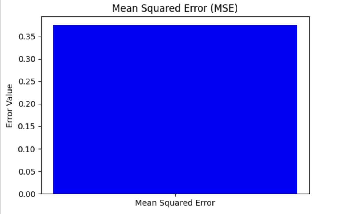
Visualize the Mean Squared Error (MSE)

To see the Mean Squared Error build a bar chart with the MSE value. This provides a clear and visual representation of the problem's magnitude.

Here, you can see how to plot it using matplotlib which is a popular Python library used for plotting −

import matplotlib.pyplot as plt
from sklearn.metrics import mean_squared_error

# Example data (replace these with your actual values)
# Actual values
y_test = [3, -0.5, 2, 7] 

# Predicted values
y_pred = [2.5, 0.0, 2, 8]  

# Calculate the MSE
mse = mean_squared_error(y_test, y_pred)

# Plotting the Mean Squared Error
plt.figure(figsize=(6, 4))
plt.bar(['Mean Squared Error'], [mse], color='blue')
plt.ylabel('Error Value')
plt.title('Mean Squared Error (MSE)')
plt.show()

Output

Here is the result of the above code −

LightGBM - Ranking

Ranking means placing elements in a specified order, like sorting students by grades or ordering search results with relevance. In machine learning, ranking is used to organize items based on their value or relevancy.

LightGBM can be used for ranking tasks which demand arranging data in an ordered manner. This is helpful in a number of events, like −

Search Engines − When you search some query on Google then the results are ordered as per their preferences with the query you have entered.
Recommended Systems − When you watch YouTube videos or shop online so the system ranks the options and proposes the ones that are most relevant to you.

Ranking Loss Functions in LightGBM

When LightGBM is used to rank, it try to put them in the most optimal order. In order to do this, LightGBM uses a "loss function." A loss function determines how well the model completes its mission. If the ranking is correct, the loss is minimal; otherwise, the loss is large. The objective is to minimize the loss function by ranking accurately as possible.

Here are some ranking loss functions we can use in LightGBM −

LambdaRank

This loss function tries to improve the relevance of search results and recommendations. This technique transforms ranking into a pairwise classification or regression problem. Basically, the algorithms evaluate a pair of items at a time to find a possible ordering for those items before starting with the final order of the complete list. LambdaRank is popular as it just ranks quality.

NDCG (Normalized Discounted Cumulative Gain)

NDCG is a statistic that finds the quality of a ranking list. It selects items near the top of the list as they are the most important. LightGBM uses NDCG as a loss function to improve its rankings. The goal is to maximize the NDCG score by displaying the most important information at the top. This is useful for search engines and recommendation systems that depend largely on the first few results.

MAP (Mean Average Precision)

Mean average precision measures how well a model performs a query. To better understand how it works, consider precision and recall, which are two often used measures for evaluating the effectiveness of a classification model. It is useful for making sure a big number of relevant items display at the top.

List-wise Loss

Instead of depending only on pairs, list-wise loss functions evaluate the entire set of rated items. This technique evaluates the overall quality of the ranking list and tries to improve it. LightGBM uses listwise loss functions to find the best ranking order for all items in a group.

Example using LightGBM for Ranking

Here is a Python code which is showing the example of LightGBM for ranking. So we will create a small dataset and then train a LightGBM model for ranking. And after that we will use it for predicting the ranking order.

Step 1 − First you have to import the necessary libraries like − lightgbm, numpy, sklearn.model_selection, and sklearn.metrics.

import lightgbm as lgb
import numpy as np
from sklearn.model_selection import train_test_split
from sklearn.metrics import ndcg_score

Step 2 − Create a sample dataset with X, y and group here X is features, y is relevance scores, and group is groups. X is the feature matrix which has seven samples and two features each. Y shows the relevance scores. Its higher value means the item is more relevant.
```
X = np.array([[0.2, 1], [0.4, 2], [0.3, 1], [0.6, 2], [0.8, 3], [0.5, 2], [0.9, 3]])
y = np.array([1, 2, 2, 3, 4, 3, 5])
group = [2, 3, 2]
```
Step 3 − Expand the group array to create a list of group indices for each sample in X. The group_indices is created by repeating the group indices for each item in its respective group.
```
group_indices = np.repeat(range(len(group)), group)
```
Step 4 − The train_test_split method splits the dataset into training and testing sets. X, y, and group_indices are splitted into training and testing sets. And we will split them in a 70:30 ratio.
```
X_train, X_test, y_train, y_test, group_train_indices, group_test_indices = train_test_split(
   X, y, group_indices, test_size=0.3, random_state=42
)
```
Step 5 − Count how many samples are in each group for the training and testing datasets. The group_train and group_test give the number of samples in each training and testing group.
```
group_train = [np.sum(group_train_indices == i) for i in np.unique(group_train_indices)]
group_test = [np.sum(group_test_indices == i) for i in np.unique(group_test_indices)]
```
Step 6 − Now we will generate LightGBM datasets for training and testing. The group parameter shows the number of samples per group which is required for ranking tasks.
```
train_data = lgb.Dataset(X_train, label=y_train, group=group_train)
test_data = lgb.Dataset(X_test, label=y_test, group=group_test)
```

Step 7 − Then we will define the parameters for the LightGBM model −

params = {
   'objective': 'lambdarank',
   'metric': 'ndcg',
   'learning_rate': 0.1,
   'num_leaves': 31,
   'min_data_in_leaf': 1,
   'ndcg_at': [1, 3, 5],
   'verbose': -1
}

Step 8 − And then train the LightGBM model with the help of the training data.

gbm = lgb.train(
   params,
   train_data,
   valid_sets=[test_data],
   num_boost_round=100,
   callbacks=[lgb.early_stopping(stopping_rounds=10)]
)

Step 9 − By using the training model to predict the test data. We have used the ndcg_score to get the performance of the model.
```
y_pred = gbm.predict(X_test)
score = ndcg_score([y_test], [y_pred])
print(f"NDCG Score: {score}")
```

Step 10 − Here is the score to understand the model ranks the test data.

Training until validation scores don't improve for 10 rounds
Early stopping, best iteration is:
[1]	valid_0's ndcg@1: 0.666667	valid_0's ndcg@3: 0.898354	valid_0's ndcg@5: 0.898354
NDCG Score: 0.894999002123018

Advantages of Using LightGBM for Ranking

Here are some benefits on why LightGBM is a great choice for ranking tasks:

Speed − LightGBM is very quick. It can handle large amounts of data easily which is essential when there are a large number of items to evaluate like thousands of products or millions of web pages. Because of its speed you get results faster so it is important for companies that need quick decisions.
Memory Efficient − LightGBM is more memory efficient than other machine learning tools. It means that the LightGBM can run on computers with less powerful hardware. It takes not much space to store data while learning what makes it best for a wide range of devices like laptops to large servers.
Accuracy − LightGBM is great at creating precise predictions. It learns the most effective method for ranking items so the final order is both accurate and useful. This high level of accuracy improves the user experience by providing the most relevant products in an online store or the top search results on a search engine.
Handles Missing Data − Sometimes your data is incomplete or contains missing values. LightGBM can handle missing data effectively without major cleanup. Even if some information is missing, the model can continue to learn from the data and make accurate ranking predictions.

LightGBM - Implementation in Python

In this chapter, we will see the steps of developing a LightGBM model in Python. We will use Scikit-learn's load_breast_cancer dataset to build a binary classification model. The steps are as follows: load the data, prepare it for LightGBM, establish the parameters, train the model, make predictions, and evaluate the outcomes.

Implementation of LightGBM

So let us create a basic model using Python −

1. Load the Dataset

First, we load the dataset with Scikit-learn's load_breast_cancer method. This dataset contains features and labels for breast cancer classification.

from sklearn.datasets import load_breast_cancer

# Load dataset
data = load_breast_cancer()
X = data.data
y = data.target

2. Split the Data

The dataset is split into training and testing sets with Scikit-learn's train_test_split method. This allows us to train the model on one set of data and then evaluate its performance on another.

from sklearn.model_selection import train_test_split

# Split the data
X_train, X_test, y_train, y_test = train_test_split(X, y, test_size=0.2, random_state=42)

3. Prepare Data for LightGBM

Convert the training and testing data into LightGBM dataset format. This step optimizes the data format for LightGBM's training algorithms.

import lightgbm as lgb

# Convert the data to LightGBM dataset format
train_data = lgb.Dataset(X_train, label=y_train)
test_data = lgb.Dataset(X_test, label=y_test, reference=train_data)

4. Define Parameters

Set the parameters of the LightGBM model. These involve the objective function, evaluation metric, learning rate, leaf count, and maximum tree depth.

params = {
    'objective': 'binary',
    'metric': 'binary_logloss',
    'boosting_type': 'gbdt',
    'learning_rate': 0.1,
    # Increased from 31
    'num_leaves': 63,  
    # Set to a positive value to limit depth
    'max_depth': 10    
}

5. Train the Model

Train the LightGBM model using the training data. To prevent overfitting, we use early stopping, which means that training ends when no progress is seen on the validation set.

# Train the model with early stopping
lgb_model = lgb.train(
    params,
    train_data,
    num_boost_round=100,
    valid_sets=[test_data],
    # Use callback for early stopping
    callbacks=[lgb.early_stopping(stopping_rounds=10)]  
)

Output

Here is the outcome of the above step −

[LightGBM] [Info] Number of positive: 286, number of negative: 169
[LightGBM] [Info] Auto-choosing col-wise multi-threading, the overhead of testing was 0.000734 seconds.
You can set `force_col_wise=true` to remove the overhead.
[LightGBM] [Info] Total Bins 4548
[LightGBM] [Info] Number of data points in the train set: 455, number of used features: 30
[LightGBM] [Info] [binary:BoostFromScore]: pavg=0.628571 -> initscore=0.526093
[LightGBM] [Info] Start training from score 0.526093
[LightGBM] [Warning] No further splits with positive gain, best gain: -inf
[LightGBM] [Warning] No further splits with positive gain, best gain: -inf

6. Make Predictions

Use the training model to predict the test data. We return the probability into binary outcomes.

# Predict on the test set
y_pred = lgb_model.predict(X_test)
y_pred_binary = [1 if x > 0.5 else 0 for x in y_pred]

7. Evaluate the Model

Calculate the accuracy score for the test set to evaluate the model's performance. This allows us to find out how well the model performs with previously unseen data.

from sklearn.metrics import accuracy_score

# Evaluate the model
accuracy = accuracy_score(y_test, y_pred_binary)
print(f"Accuracy: {accuracy:.2f}")

Output

Here is the accuracy of the above model −

Accuracy: 0.96

Exploratory Data Analysis (EDA) for the LightGBM Model

Exploratory Data Analysis (EDA) must be done before training and testing the LightGBM model in order to understand the dataset, identify patterns, and prepare it for modeling. EDA involves examining the dataset's structure, distributions, correlations, and potential issues.

Here are the steps on using EDA for the load_breast_cancer dataset −

1. Load and Inspect the Dataset

First we have to load the dataset and inspect its basic structure like the number of samples, features, and target variable.

import pandas as pd
from sklearn.datasets import load_breast_cancer

# Load dataset
data = load_breast_cancer()
df = pd.DataFrame(data.data, columns=data.feature_names)
df['target'] = data.target

# Inspect the dataset
print(df.head())
print(df.info())
print(df.describe())

Output

This will lead to the following outcome:

   mean radius  mean texture  mean perimeter  mean area  mean smoothness  \
0        17.99         10.38          122.80     1001.0          0.11840   
1        20.57         17.77          132.90     1326.0          0.08474   
2        19.69         21.25          130.00     1203.0          0.10960   
3        11.42         20.38           77.58      386.1          0.14250   
4        20.29         14.34          135.10     1297.0          0.10030   

   mean compactness  mean concavity  mean concave points  mean symmetry  \
0           0.27760          0.3001              0.14710         0.2419   
1           0.07864          0.0869              0.07017         0.1812   
2           0.15990          0.1974              0.12790         0.2069   
3           0.28390          0.2414              0.10520         0.2597   
4           0.13280          0.1980              0.10430         0.1809   

   mean fractal dimension  ...  worst texture  worst perimeter  worst area  \
0                 0.07871  ...          17.33           184.60      2019.0   
1                 0.05667  ...          23.41           158.80      1956.0   
2                 0.05999  ...          25.53           152.50      1709.0   
3                 0.09744  ...          26.50            98.87       567.7   
4                 0.05883  ...          16.67           152.20      1575.0   

   worst smoothness  worst compactness  worst concavity  worst concave points  \
0            0.1622             0.6656           0.7119                0.2654   
1            0.1238             0.1866           0.2416                0.1860   
2            0.1444             0.4245           0.4504                0.2430   
3            0.2098             0.8663           0.6869                0.2575   
4            0.1374             0.2050           0.4000                0.1625   

   worst symmetry  worst fractal dimension  target  
0          0.4601                  0.11890       0  
1          0.2750                  0.08902       0  
2          0.3613                  0.08758       0  
3          0.6638                  0.17300       0  
4          0.2364                  0.07678       0

2. Check for Missing Values

Now let us see are there any missing values in the dataset.

# Check for missing values
print(df.isnull().sum())

Output

This will generate the below result:

mean radius                0
mean texture               0
mean perimeter             0
mean area                  0
mean smoothness            0
mean compactness           0
mean concavity             0
mean concave points        0
mean symmetry              0
mean fractal dimension     0
radius error               0
texture error              0
perimeter error            0
area error                 0
smoothness error           0
compactness error          0
concavity error            0
concave points error       0
symmetry error             0
fractal dimension error    0
worst radius               0
worst texture              0
worst perimeter            0
worst area                 0
worst smoothness           0
worst compactness          0
worst concavity            0
worst concave points       0
worst symmetry             0
worst fractal dimension    0
target                     0
dtype: int64

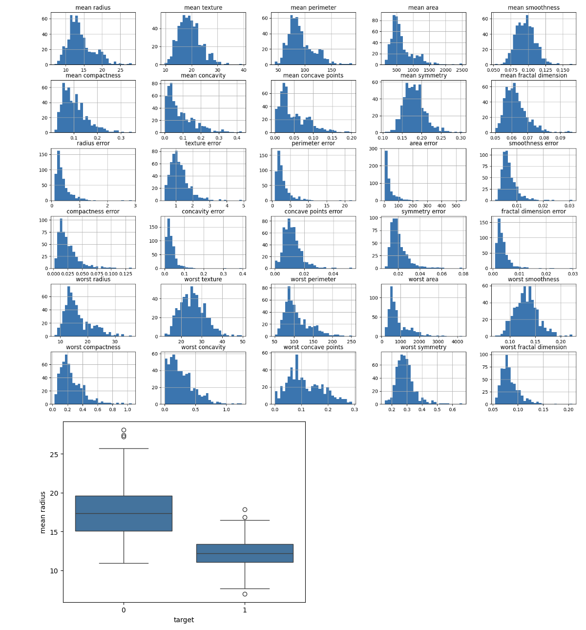
3. Feature Distributions

Determine the distribution of each feature. To understand more about the range and distribution of feature values, use histograms, box plots, or other visualizations.

import matplotlib.pyplot as plt
import seaborn as sns

# Plot histograms for each feature
df.iloc[:, :-1].hist(bins=30, figsize=(20, 15))
plt.show()

# Box plot for a selected feature
sns.boxplot(x='target', y='mean radius', data=df)
plt.show()

Output

This will create the below outcome:

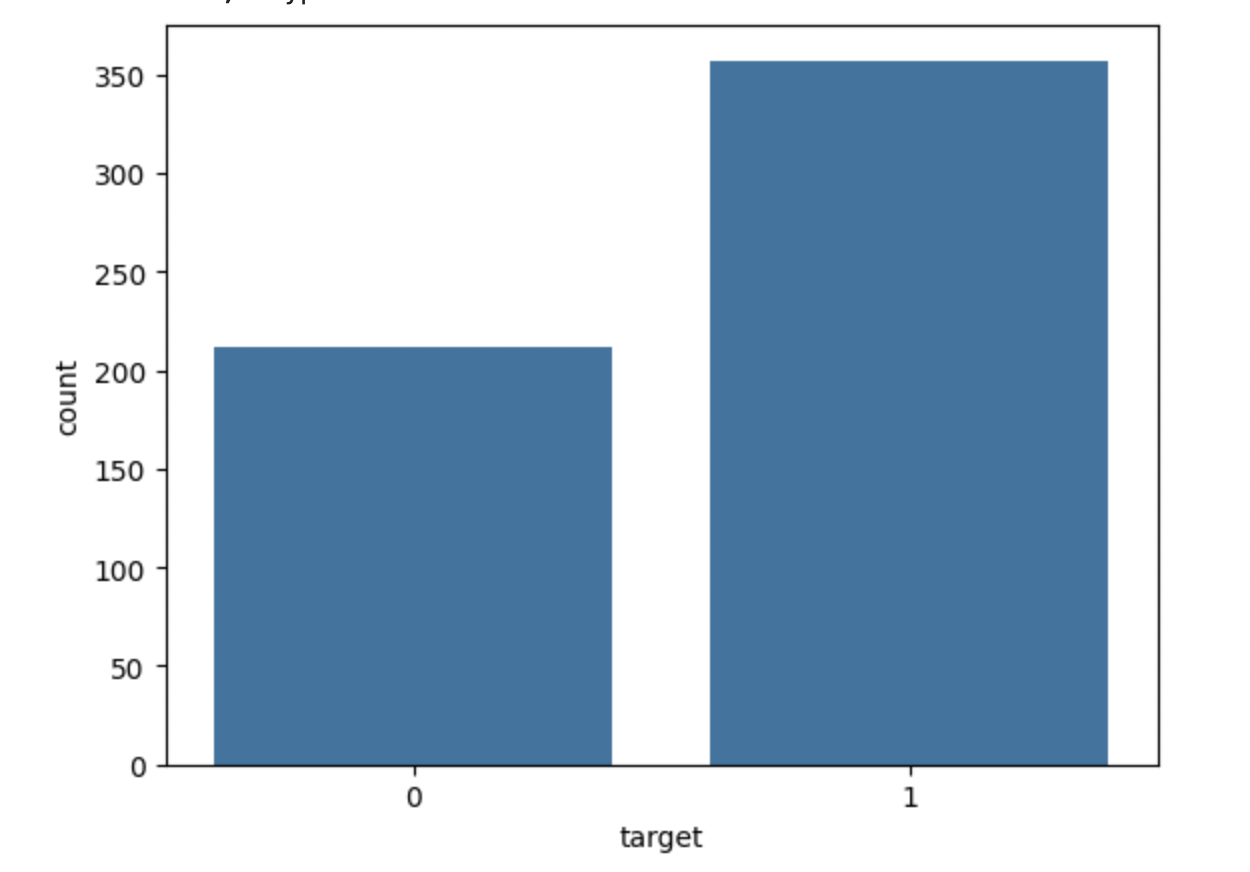
4. Analyze Class Distribution

Check the distribution of the target variable to find the class balance. This will allow you to identify if the dataset is imbalanced.

# Class distribution
print(df['target'].value_counts())
sns.countplot(x='target', data=df)
plt.show()

Output

This will show the below output −

target
1    357
0    212
Name: count, dtype: int64

Summary

Following these steps will allow you to create and test a LightGBM model for classification problems in Python. This technique can be modified for different datasets and problems by adjusting the parameters and preparation steps as needed.

LightGBM - Parameter Tuning

Optimizing LightGBM's parameters is essential for boosting the model's performance, both in terms of speed and accuracy. This chapter describes in detail how to adjust the most necessary LightGBM parameters.

What is Parameter Tuning ?

Parameter tuning is the process of adjusting a machine learning model's hyperparameters or parameters to maximize performance. In models like LightGBM, hyperparameters that control a model's learning process are leaf count, learning rate, and tree depth.

The parameters are required because −

Boosts Accuracy − On new, untested data, a fine-tuned model generates predicts that are more accurate.
Prevents Overfitting/Underfitting − It ensures that the model is neither too complex nor too simple.
Optimizes Speed − Tuning can reduce training times without affecting performance by using less memory or processor power.

So Let us see how we can tune the parameters of the LightGBM model −

1. Controlling Model Complexity

These are methods for regulating model complexity, balancing underfitting and overfitting by adjusting parameters like as num_leaves and max_depth. Tuning these parameters help us to manage the complexity of the LightGBM model.

num_leaves − It is used to control the number of leaves in each decision tree. More leaves increase model complexity, but too many can lead to overfitting. Set num_leaves less than or equal to 2^(max_depth). For example, if max_depth = 6, set num_leaves <= 64.
min_data_in_leaf − Displays the minimum number of samples, or data points, that a leaf can include. By changing this parameter, you can help the model reduce noise in the data. If the depth is too low, the tree could grow too deeply and become overfit. Values in the hundreds or thousands range are good for large datasets.
max_depth − It is used to limit the depth of the tree. This can help prevent overfitting by limiting the depth to which the trees can grow. So use in combination with num_leaves to control the tree's complexity.

2. Speeding Up the Model

Training speed can be increased without compromising accuracy by using methods like bagging, feature sub-sampling, and max_bin reduction.

Bagging − To speed up training, use a subset of the data in each cycle. By setting the parameters.The percentage of data to be used in each iteration is given by the variable bagging_fraction. The bagging_freq returns the number of bagging iterations per frequency. Two suitable settings to set are bagging_fraction = 0.8 and bagging_freq = 5 to accelerate the model without significantly affecting accuracy.
Feature Sub-sampling − Randomly selects a subset of features to train at each iteration. Use the parameters like feature_fraction. This parameter controls the fraction of features to be used for training. For best practice set feature_fraction = 0.8 to reduce training time.
max_bin − This parameter controls the number of bins used for continuous features. So the best practice is that the max_bin can be decreased to speed up the model and consume less memory, but accuracy can be compromised.
save_binary − Binary data is stored in order to allow faster loading in successive runs. So it is advised to use save_binary=True when running the model repeatedly on the same dataset.

3. Improving Accuracy

Using larger datasets, lower learning rates, and advanced techniques like Dart can improve the model's accuracy, but can come at the cost of longer training durations.

learning_rate and num_iterations − The number of steps and quantity of model modifications made at each iteration are controlled by the parameters learning_rate and num_iterations. Using a smaller learning_rate (like 0.01) and a greater num_iterations (like 1000+) is the best option.
num_leaves − Increased num_leaves makes the model more complex. This may increase accuracy, but if used incorrectly, it may also lead to overfitting. So the best practice is to increase num_leaves if you have enough data, but make sure to combine it with regularization techniques to avoid overfitting.
Training with Bigger Data − More data usually leads to higher accuracy because the model can pick up on a larger range of patterns. So the best practice is to improve the model's ability to generalize, use as much data as possible if overfitting is an issue.
Dart (Dropouts meet Multiple Additive Regression Trees) − This particular version of the gradient boosting technique increases the model's accuracy by randomly deleting trees during training. Therefore, the best practice is to use boosting_type='dart' for issues where you see overfitting or if you are looking for an extra accuracy.
Using Categorical Features − By removing the need to convert categorical features into dummy variables, LightGBM can handle them directly, potentially increasing performance. Therefore, it is better to improve model accuracy by using the categorical_feature option to identify which attributes are categorical.

4. Handling Overfitting

This section explains how subsampling techniques, tree depth restrictions, and regularization are used to prevent the model from overfitting the training set.

max_bin − Using a smaller max_bin can reduce overfitting because it limits the amount of detail in feature binning.
num_leaves − To prevent the training set from being overfit and the model from growing too complicated, decrease the number of leaves in the model.
min_data_in_leaf and min_sum_hessian_in_leaf − These settings help prevent the tree from going too deep by ensuring that each leaf contains a minimum sum of the second derivative (min_sum_hessian_in_leaf) and a minimum amount of data points (min_data_in_leaf). Increase the min_data_in_leaf and min_sum_hessian_in_leaf to avoid overfitting, particularly for small datasets.
Bagging and Feature Sub-sampling − Use feature sub-sampling (feature_fraction) and bagging (bagging_fraction and bagging_freq) to increase unpredictability in the model and reduce overfitting.
Regularization − Defining parameters like lambda_l1 which is L1 regularization, commonly referred to as Lasso, to reduce the complexity of the model. And lambda_l2 is used to reduce overfitting with ridge-based L2 regularization. The minimal gain required to split a tree node is indicated by the variable min_gain_to_split. Try increasing lambda_l1 and lambda_l2 to add regularization to the model, and adjust min_gain_to_split to control how easily the model creates new branches.
max_depth − Set a reasonable max_depth to limit the depth of the trees and avoid overfitting, especially on smaller datasets.

Example of Parameter Tuning in Python

Here is the small example for performing LightGBM parameter tuning in Python −

# Import necessary libraries
import pandas as pd
import numpy as np
import matplotlib.pyplot as plt
import seaborn as sns

from sklearn.model_selection import train_test_split, RandomizedSearchCV
import lightgbm as lgb
from sklearn.metrics import accuracy_score, classification_report, confusion_matrix

sns.set(style="whitegrid", color_codes=True, font_scale=1.3)

import warnings
warnings.filterwarnings('ignore')

# Load dataset
data = pd.read_csv('/Python/breast_cancer_data.csv')
data.head()

# 1. Preprocessing
# Drop unnecessary columns
data = data.drop(columns=['id', 'Unnamed: 32'])

# Convert 'diagnosis' column to numerical (0: Benign, 1: Malignant)
data['diagnosis'] = data['diagnosis'].map({'B': 0, 'M': 1})

# Split the data into features (X) and target (y)
X = data.drop(columns=['diagnosis'])
y = data['diagnosis']

# Clean column names to avoid LightGBM error
X.columns = X.columns.str.replace('[^A-Za-z0-9_]+', '', regex=True)

# Train-test split
X_train, X_test, y_train, y_test = train_test_split(X, y, test_size=0.2, random_state=42)

# 2. Define parameter grid for tuning
param_grid = {
    'learning_rate': [0.01, 0.05, 0.1],
    'num_leaves': [20, 31, 40],
    'max_depth': [-1, 10, 20],
    'feature_fraction': [0.6, 0.8, 1.0],
    'bagging_fraction': [0.6, 0.8, 1.0],
    'bagging_freq': [0, 5, 10],
    'lambda_l1': [0, 1, 5],
    'lambda_l2': [0, 1, 5]
}

# 3. Set up the LightGBM model
lgb_estimator = lgb.LGBMClassifier(objective='binary', metric='binary_logloss')

# 4. Perform Randomized Search for parameter tuning
random_search = RandomizedSearchCV(estimator=lgb_estimator, param_distributions=param_grid, 
                                   n_iter=50, scoring='accuracy', cv=5, verbose=1, random_state=42)

# 5. Fit the model
random_search.fit(X_train, y_train)

# 6. Get the best parameters
print("Best Parameters:", random_search.best_params_)

# 7. Predict and evaluate the model
y_pred = random_search.predict(X_test)
accuracy = accuracy_score(y_test, y_pred)
print(f"Accuracy: {accuracy * 100:.2f}%")

# Confusion Matrix
conf_matrix = confusion_matrix(y_test, y_pred)
print("Confusion Matrix:")
print(conf_matrix)

# Classification report
print("Classification Report:")
print(classification_report(y_test, y_pred))

# Optional: Plot Confusion Matrix for visualization
plt.figure(figsize=(8,6))
sns.heatmap(conf_matrix, annot=True, fmt='d', cmap='Blues', xticklabels=['Benign', 'Malignant'], yticklabels=['Benign', 'Malignant'])
plt.xlabel('Predicted')
plt.ylabel('Actual')
plt.title('Confusion Matrix')
plt.show()

Output

Here is the output of the above parameter tuning of LightGBM model −

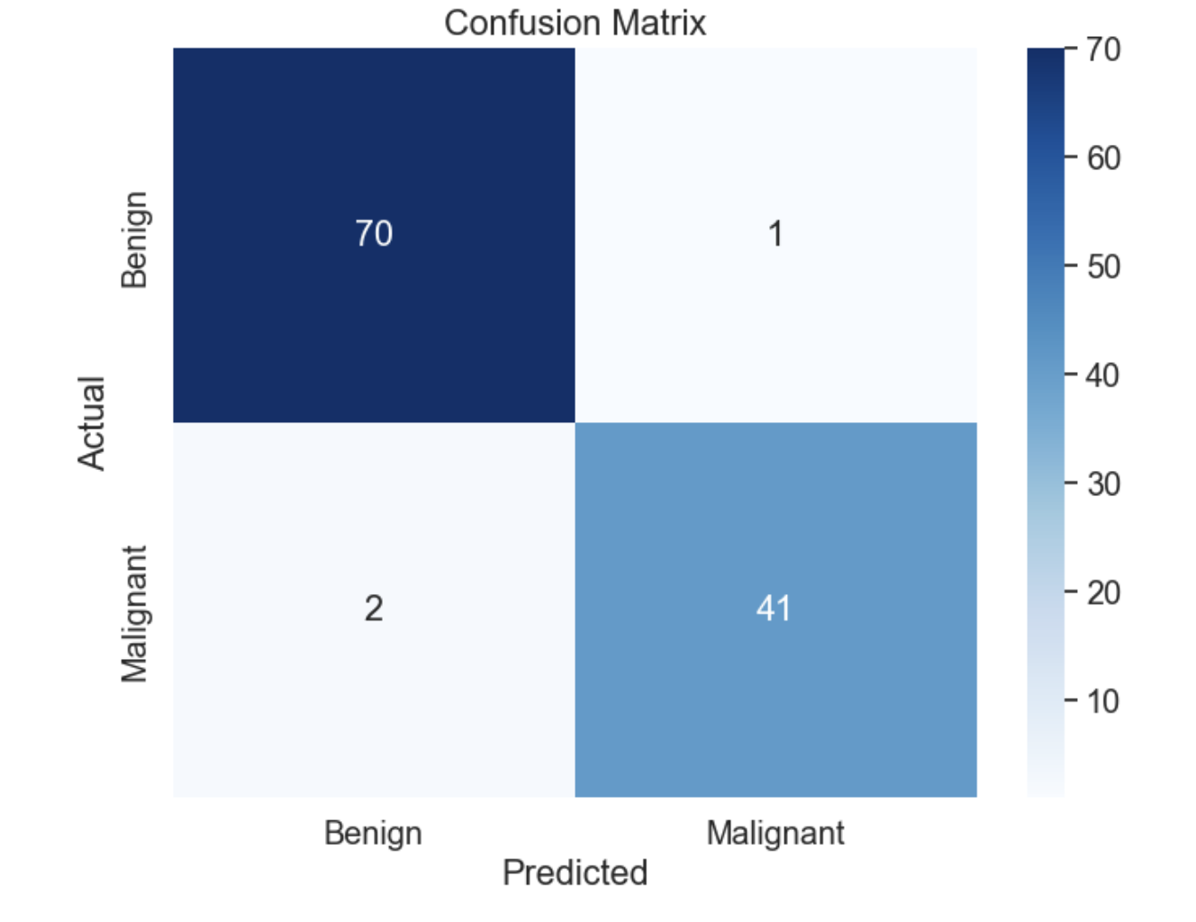
Accuracy: 97.37%
Confusion Matrix:
[[70  1]
 [ 2 41]]
Classification Report:
              precision    recall  f1-score   support

           0       0.97      0.99      0.98        71
           1       0.98      0.95      0.96        43

    accuracy                           0.97       114
   macro avg       0.97      0.97      0.97       114
weighted avg       0.97      0.97      0.97       114

The confusion matrix is as follows −

Summary

LightGBM parameters need to be tuned in order to maximize model performance and training speed. Finding a balance between speed, precision, complexity, and overfitting prevention is key. By carefully adjusting parameters like num_leaves, min_data_in_leaf, bagging_fraction, and max_depth, you can build a model that performs well on both training and unseen data. Here, L1 and L2 regularization procedures can help further prevent overfitting and enhance the model's generalization.

LightGBM - Plotting Functionality

LightGBM offers various tools for creating plots that help you visualize the performance of your models, feature importance, and more. So in this chapter we are writing some common plotting functions you can use with LightGBM.

LightGBM Plotting Functions

So here is a list of plotting functions commonly used in LightGBM −

plot_importance()

The plot_importance() method uses a booster object and then plot the feature importance. This method uses a parameter called importance_type which is used to set to string split and it will plot the number of times feature is used for splitting and plotting gains of splits when it is set to string gain. The value of the parameter importance_type is split.

The function has one more parameter called max_num_features and it accepts an integer which shows how many features we need to include in the plot. Also we can limit the number of features with the help of this parameter.

Syntax

Here is the syntax we can use for the plot_importance() function −

lightgbm.plot_importance(
   ax=None, 
   booster, 
   height=0.2, 
   ylim=None, 
   xlim=None, 
   xlabel='Feature importance', 
   title='Feature importance', 
   importance_type='split', 
   ylabel='Features', 
   ignore_zero=True, 
   max_num_features=None, 
   grid=True, 
   figsize=None, 
   precision=3
)

Parameters

The parameters are needed to use the plot_importance() function are mentioned below −

booster − It is the trained LightGBM model.
importance_type − It is used to define how to calculate feature importance. It has two values split and gain. The default value is split.
max_num_features − Used to Limit the number of top features.
figsize − It is a tuple and used to show the size of the plot, for example (10, 6).
xlabel, ylabel − These are the labels for the x and y axes.
title − It defines the title for the plot.
ignore_zero − If it is set to True it basically ignores features with zero importance.
grid − If it is set to True so it displays the grid in the plot.

Example

Here is the example shown below to show you the usage of plot_importance() function −

import lightgbm as lgb
import matplotlib.pyplot as plt

# Assuming you have a trained model `gbm`
lgb.plot_importance(gbm, importance_type='gain', max_num_features=10, figsize=(10, 6))
plt.show()

Output

Here is the output of the above code −

plot_metric()

The plot_metric() function is used to plot the results of an evaluation metric. To use this function we have to give a booster object inside the method to plot an evaluation metric evaluated on the dataset.

Syntax

Below is the syntax we can use for the plot_metric() function −

lightgbm.plot_metric(
   eval_result, 
   metric=None, 
   dataset_names=None, 
   ax=None, 
   title='Metric during training', 
   xlabel='Iterations', 
   ylabel='Auto', 
   figsize=None, 
   grid=True
)

Parameters

Here are the parameters needed for the plot_metric() function −

eval_result − It is a dictionary which is returned by the train() method. It basically contains the evaluation results.
metric − It is the evaluation metric that you want to plot. It is none so all metrics are plotted.
dataset_names − It is the list of dataset names to use in the plot.
ax − It is the Matplotlib axes object to plot. If it is set to None so a new plot is created.
title − It is the title of the plot.
xlabel − It is the label for the X-axis.
ylabel − It is the label for the Y-axis.
figsize − It is the tuple for the figure size.
grid − It is used to show a grid. Its default value is True.

Example

Here is the Python complete code which uses the model and shows the usage of plot_metric() function −

import lightgbm as lgb
import matplotlib.pyplot as plt
from sklearn.datasets import make_blobs
from sklearn.model_selection import train_test_split

# Generate sample binary classification data
X, y = make_blobs(n_samples=10_000, centers=2)

# Split the data 
X_train, X_valid, y_train, y_valid = train_test_split(X, y, train_size=0.8)

# Prepare the dataset for LightGBM
dtrain = lgb.Dataset(X_train, label=y_train)
dvalid = lgb.Dataset(X_valid, label=y_valid)

# Dictionary to store results
evals_result = {}

# Train the model 
model = lgb.train(
   params={
      "objective": "binary",
      "metric": "auc",  
   },
   train_set=dtrain,
   valid_sets=[dvalid],
   valid_names=['valid'], 
   num_boost_round=10,
   callbacks=[
      lgb.early_stopping(stopping_rounds=3),
      lgb.record_evaluation(evals_result)  
   ]
)

# Plot the evaluation metric 
lgb.plot_metric(evals_result, metric='auc')
plt.show()

Output

Following is the outcome of the mentioned code −

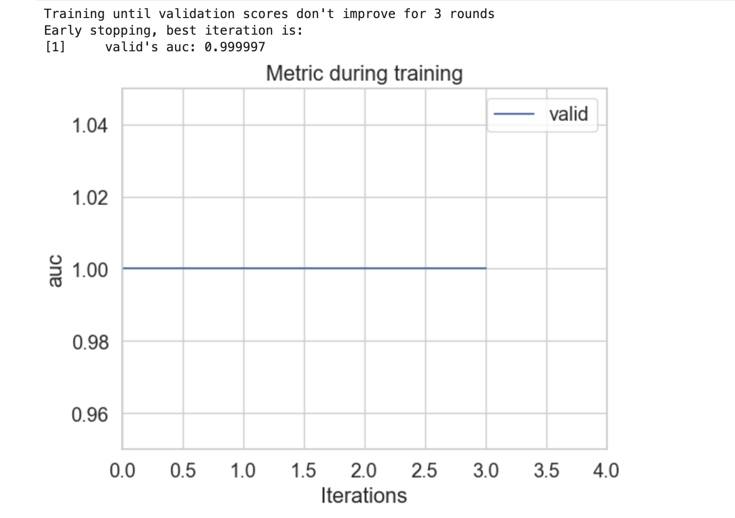
plot_split_value_histogram()

The plot_split_value_histogram() function basically accepts an input booster object and feature name/index. After that it plots a split value histogram for the given feature.

Syntax

Here is the syntax you can use for plot_split_value_histogram() function −

lightgbm.plot_split_value_histogram(
   booster, 
   feature, 
   bins=100, 
   ax=None, 
   width_coef=0.8, 
   xlim=None, 
   ylim=None, 
   title=None, 
   xlabel=None, 
   ylabel=None, 
   figsize=None, 
   dpi=None, 
   grid=False, 
)

Parameters

Here are the required and optional parameters of the plot_split_value_histogram() function:

booster − It is the trained LightGBM model also known as booster object.
feature − It is the name of the feature that you want to plot.
bins − It is the number of bins you can use for the histogram.
ax − It is the Matplotlib axes object which is optional. If it is given the plot will be drawn on this axes.
width_coef − It is coefficient for managing the width of the bars in the histogram.
xlim − It is the tuple for x-axis limit.
ylim − It is the tuple for y-axis limits.
title − It is the title of the plot.
xlabel − It is the label for the x-axis.
ylabel − It is the label for the y-axis.
figsize − It is the tuple for the size of the figure.
dpi − It is the dots per inch for the plot.
grid − This parameter uses the Boolean value to show a grid in the plot.

Example

Here is the way you can include the plot_split_value_histogram() function and see the result −

# Complete code is similar to the above mentioned example for plot_metric()
# Plot the split value histogram 
lgb.plot_split_value_histogram(model, feature=feature_to_plot)
plt.show()

Output

This will create the below outcome:

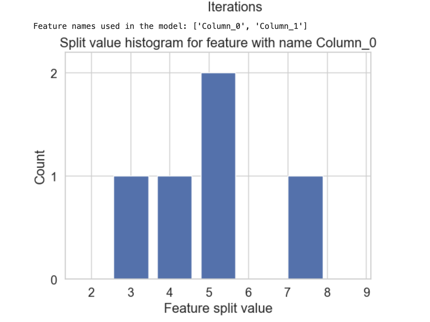
LightGBM plot_split_value_histogram() Function

plot_tree()

The plot_tree() function allows you to plot the single tree of the ensemble. For this we have to mention a booster object with the index of the tree for which we have to plot to it.

Syntax

Here is the syntax you can use for plot_split_value_histogram() function −

lightgbm.plot_tree(
   booster, 
   tree_index=0, 
   figsize=(10, 10),
   dpi=None, 
   show_info=True, 
   precision=3,
   orientation='horizontal',
   example_case=None,
)

Parameters

Here are the required and optional parameters of the plot_split_value_histogram() function:

booster − It is the booster or LGBMModel object which is to be plotted.
tree_index − It is the target axes object. If it is None then new figure and axes is created.
figsize − It is the index of a target tree to plot.
dpi − It is the resolution of the figure.
show_info − It is used to display additional information about each node in the tree.
precision − It is used to restrict the display of floating point values to a certain precision.
orientation − It is the orientation of the tree. Its value can be horizontal or vertical.
example_case − It is the single row which has the same structure as the training data.

create_tree_digraph()

The create_tree_digraph() method is used to display the structure of a given decision tree from a LightGBM model. It basically generates a graph which shows how the tree splits data at every node which makes it easy to understand the decision-making process of the model.

Syntax

Here is the syntax you can use for create_tree_digraph() function −

lightgbm.create_tree_digraph(
   booster, 
   tree_index=0, 
   show_info=None, 
   precision=3, 
   orientation='horizontal', 
   example_case=None, 
   max_category_values=10
)

Parameters

Here are the required and optional parameters of the create_tree_digraph() function:

booster − It is the booster or LGBMModel object to be converted.
tree_index − It is the index of a target tree to convert.
show_info − It is the information which should be shown in nodes. The values can be split_gain, internal_value, internal_count, internal_weight, leaf_count, leaf_weight and data_percentage.
precision − It is used to limit the display of floating-point values to a specific precision.
orientation − It is the orientation of the tree. The values can be horizontal or vertical.
example_case − It is the single row with the same structure as the training data.
max_category_values − It is the maximum number of category values to show in tree nodes. If the value of thresholds is larger than this value, it will be collapsed and shown on the label tooltip instead.

LightGBM - Early Stopping Training

Early stopping training is a method in which we finish training if the evaluation metric assessed on the evaluation dataset does not improve after a particular number of cycles. Lightgbm's sklearn-like estimators have a parameter named early_stopping_rounds in both the train() and fit() methods. This parameter accepts an integer value stating that the training process should be stopped if the evaluation metric result has not improved after a certain number of rounds.

This parameter accepts an integer value which shows that the training process should be terminated if the evaluation metric result does not improve after several rounds.

So keep in mind that this requires an evaluation dataset to work because it relies on evaluation metric results that are assessed against the evaluation dataset.

Example

We will first import the necessary libraries before loading the Boston housing dataset. As of version 1.2 the dataset is no longer available in Scikit-Learn so we will either replicate the feature using sklearn.datasets.load_boston().

from sklearn.model_selection import train_test_split

X_train, X_test, Y_train, Y_test = train_test_split(boston.data, boston.target)

print("Sizes of Train or Test Datasets : ", X_train.shape, X_test.shape, Y_train.shape, Y_test.shape)

train_dataset = lgb.Dataset(X_train, Y_train, feature_name=boston.feature_names.tolist())
test_dataset = lgb.Dataset(X_test, Y_test, feature_name=boston.feature_names.tolist())

booster = lgb.train({"objective": "regression", "verbosity": -1, "metric": "rmse"},
                    train_set=train_dataset, valid_sets=(test_dataset,),
                    early_stopping_rounds=5,
                    num_boost_round=100)

from sklearn.metrics import r2_score

test_preds = booster.predict(X_test)
train_preds = booster.predict(X_train)

# Display the R2 scores in the console
print("\nR2 Score on Test Set : %.2f"%r2_score(Y_test, test_preds))
print("R2 Score on Train Set : %.2f"%r2_score(Y_train, train_preds))

Output

This will produce the following result:

Sizes of Train or Test Datasets:  (404, 13) (102, 13) (404,) (102,)
[1]	valid_0's rmse: 9.10722
Training until validation scores don't improve for 5 rounds
[2]	valid_0's rmse: 8.46389
[3]	valid_0's rmse: 7.93394
[4]	valid_0's rmse: 7.43812
[5]	valid_0's rmse: 7.01845
[6]	valid_0's rmse: 6.68186
[7]	valid_0's rmse: 6.43834
[8]	valid_0's rmse: 6.17357
[9]	valid_0's rmse: 5.96725
[10]	valid_0's rmse: 5.74169
[11]	valid_0's rmse: 5.55389
[12]	valid_0's rmse: 5.38595
[13]	valid_0's rmse: 5.24832
[14]	valid_0's rmse: 5.13373
[15]	valid_0's rmse: 5.0457
[16]	valid_0's rmse: 4.96688
[17]	valid_0's rmse: 4.87874
[18]	valid_0's rmse: 4.8246
[19]	valid_0's rmse: 4.75342
[20]	valid_0's rmse: 4.69854
Did not meet early stopping. Best iteration is:
[20]	valid_0's rmse: 4.69854

R2 Score on Test Set: 0.81
R2 Score on Train Set: 0.97

This program divides the breast cancer dataset into two sections like training and testing. It trains a LightGBM model to decide whether a tumor is dangerous or harmless so stopping early if performance fails to improve. Finally it predicts the results for both the test and training sets and computes accuracy of the model.

from sklearn.model_selection import train_test_split

X_train, X_test, Y_train, Y_test = train_test_split(breast_cancer.data, breast_cancer.target)

print("Sizes of Train or Test Datasets : ", X_train.shape, X_test.shape, Y_train.shape, Y_test.shape)

booster = lgb.LGBMModel(objective="binary", n_estimators=100, metric="auc")

booster.fit(X_train, Y_train,
            eval_set=[(X_test, Y_test),],
            early_stopping_rounds=3)

from sklearn.metrics import accuracy_score

test_preds = booster.predict(X_test)
train_preds = booster.predict(X_train)

test_preds = [1 if pred > 0.5 else 0 for pred in test_preds]
train_preds = [1 if pred > 0.5 else 0 for pred in train_preds]

# Display the accuracy results
print("\nAccuracy Score on Test Set : %.2f"%accuracy_score(Y_test, test_preds))
print("Accuracy Score on Train Set : %.2f"%accuracy_score(Y_train, train_preds))

Output

This will lead to the following outcome:

Sizes of Train or Test Datasets :  (426, 30) (143, 30) (426,) (143,)
[1]	valid_0's auc: 0.986129
Training until validation scores don't improve for 3 rounds
[2]	valid_0's auc: 0.989355
[3]	valid_0's auc: 0.988925
[4]	valid_0's auc: 0.987097
[5]	valid_0's auc: 0.990108
[6]	valid_0's auc: 0.993011
[7]	valid_0's auc: 0.993011
[8]	valid_0's auc: 0.993441
[9]	valid_0's auc: 0.993441
[10]	valid_0's auc: 0.994194
[11]	valid_0's auc: 0.994194
[12]	valid_0's auc: 0.994194
[13]	valid_0's auc: 0.994409
[14]	valid_0's auc: 0.995914
[15]	valid_0's auc: 0.996129
[16]	valid_0's auc: 0.996989
[17]	valid_0's auc: 0.996989
[18]	valid_0's auc: 0.996344
[19]	valid_0's auc: 0.997204
[20]	valid_0's auc: 0.997419
[21]	valid_0's auc: 0.997849
[22]	valid_0's auc: 0.998065
[23]	valid_0's auc: 0.997849
[24]	valid_0's auc: 0.998065
[25]	valid_0's auc: 0.997634
Early stopping, best iteration is:
[22]	valid_0's auc: 0.998065

Accuracy Score on Test Set : 0.97
Accuracy Score on Train Set : 0.98

How to stop training early through the "early_stopping()" callback?

LightGBM actually supports early-stopping training using the early_stopping() callback mechanism. We can give the number of rounds for the early_stopping() function as a callback argument to the train()/fit() method. Usage of callbacks is given below −

from sklearn.model_selection import train_test_split

X_train, X_test, Y_train, Y_test = train_test_split(breast_cancer.data, breast_cancer.target)

print("Sizes of Train or Test Datasets : ", X_train.shape, X_test.shape, Y_train.shape, Y_test.shape)

booster = lgb.LGBMModel(objective="binary", n_estimators=100, metric="auc")

booster.fit(X_train, Y_train,
            eval_set=[(X_test, Y_test),],
            callbacks=[lgb.early_stopping(3)]
            )

from sklearn.metrics import accuracy_score

test_preds = booster.predict(X_test)
train_preds = booster.predict(X_train)

test_preds = [1 if pred > 0.5 else 0 for pred in test_preds]
train_preds = [1 if pred > 0.5 else 0 for pred in train_preds]

print("\nAccuracy Score on Test Set : %.2f"%accuracy_score(Y_test, test_preds))
print("Accuracy Score on Train Set : %.2f"%accuracy_score(Y_train, train_preds))

Output

This will generate the below result:

Sizes of Train or Test Datasets :  (426, 30) (143, 30) (426,) (143,)
[1]	valid_0's auc: 0.954328
Training until validation scores don't improve for 3 rounds
[2]	valid_0's auc: 0.959322
[3]	valid_0's auc: 0.982938
[4]	valid_0's auc: 0.988244
[5]	valid_0's auc: 0.987203
[6]	valid_0's auc: 0.98762
[7]	valid_0's auc: 0.98814
Early stopping, best iteration is:
[4]	valid_0's auc: 0.988244

Accuracy Score on Test Set : 0.94
Accuracy Score on Train Set : 0.95

LightGBM - Feature Interaction Constraints

When lightgbm has finished training the ensemble trees on a dataset, each node denotes a condition determined by a feature value. When making predictions with an individual tree, we start at the root node and compare the feature condition given in the node to our sample feature values. We make decisions as per the feature values in our sample and the condition of the tree. This allows us to generate the final prediction by taking a specific path to the leaf of the tree. By default there are no limitations on which nodes can have which capability.

This method of generating a final decision by iterating over nodes of a tree and analyzing feature condition is known as feature interaction, because the predictor arrived to the specific node after evaluating the state of the previous one. LightGBM allows us to decide which features can interact with each other. We can define a set of indices and only those qualities will interact with one another. These features will be unable to interact with other features and this limitation will be enforced when trees are generated during the training phase.

We have shown how to force a feature interaction constraints on an estimator in LightGBM. LightGBM estimators have a parameter called interaction_constraints which accepts a list of lists each containing indices of parameters that can interact with one another.

Example 1

Here is an example of how we can force Feature Interaction Constraint on estimator in lightgbm.

The load_boston function from sklearn.datasets may be deprecated in some versions of scikit-learn. If any error occurs than you can load the dataset from an external source or use an alternative dataset.

# Import necessary libraries
import lightgbm as lgb
from sklearn.datasets import load_boston
from sklearn.model_selection import train_test_split
from sklearn.metrics import r2_score

# Load the Boston housing dataset
boston = load_boston()

# Split the data into training and testing sets
X_train, X_test, Y_train, Y_test = train_test_split(boston.data, boston.target, train_size=0.90, random_state=42)

# Print the size of the training and testing sets
print("Sizes of Train or Test Datasets : ", X_train.shape, X_test.shape, Y_train.shape, Y_test.shape, "\n")

# Create LightGBM datasets
train_dataset = lgb.Dataset(X_train, Y_train, feature_name=boston.feature_names.tolist())
test_dataset = lgb.Dataset(X_test, Y_test, feature_name=boston.feature_names.tolist())

# Train the LightGBM model
booster = lgb.train({
    "objective": "regression",
    "verbosity": -1,
    "metric": "rmse",
    'interaction_constraints': [[0,1,2,11,12], [3,4], [6,10], [5,9], [7,8]]
    },
    train_set=train_dataset,
    valid_sets=(test_dataset,),
    num_boost_round=10
)

# Make predictions
test_preds = booster.predict(X_test)
train_preds = booster.predict(X_train)

# Calculate and print R2 scores
print("\nR2 Test Score : %.2f" % r2_score(Y_test, test_preds))
print("R2 Train Score : %.2f" % r2_score(Y_train, train_preds))

Output

This will generate the below result:

Sizes of Train or Test Datasets :  (455, 13) (51, 13) (455,) (51,)

[1]	valid_0's rmse: 7.50225
[2]	valid_0's rmse: 7.01989
[3]	valid_0's rmse: 6.58246
[4]	valid_0's rmse: 6.18581
[5]	valid_0's rmse: 5.83873
[6]	valid_0's rmse: 5.47166
[7]	valid_0's rmse: 5.19667
[8]	valid_0's rmse: 4.96259
[9]	valid_0's rmse: 4.69168
[10]	valid_0's rmse: 4.51653

R2 Test Score : 0.67
R2 Train Score : 0.69

Example 2

Now the below code trains a LightGBM model to predict housing prices using the Boston dataset. After training it will calculate how well the model works on both the training and test data using the R² score.

# Import necessary libraries
import lightgbm as lgb
from sklearn.datasets import load_boston
from sklearn.model_selection import train_test_split
from sklearn.metrics import r2_score

# Load the Boston housing dataset
boston = load_boston()

# Split the dataset into training and testing sets
X_train, X_test, Y_train, Y_test = train_test_split(boston.data, boston.target, test_size=0.2, random_state=42)

# Print the size of the training and testing sets
print("Sizes of Training and Testing Datasets : ", X_train.shape, X_test.shape, Y_train.shape, Y_test.shape)

# Create a LightGBM model with interaction constraints and 10 estimators
booster = lgb.LGBMModel(objective="regression", n_estimators=10,
                        interaction_constraints=[[0,1,2,11,12], [3, 4], [6,10], [5,9], [7,8]])

# Train the model on the training set and validate it on the test set
booster.fit(X_train, Y_train,
            eval_set=[(X_test, Y_test)],
            eval_metric="rmse")

# Make predictions on both the test and training sets
test_preds = booster.predict(X_test)
train_preds = booster.predict(X_train)

# Calculate and print the R2 score for the test and training sets
print("\nR2 Test Score : %.2f" % r2_score(Y_test, test_preds))
print("R2 Train Score : %.2f" % r2_score(Y_train, train_preds))

Output

This will create the following result:

Sizes of Training and Testing Datasets :  (379, 13) (127, 13) (379,) (127,)
[1]	valid_0's rmse: 8.97871	valid_0's l2: 80.6173
[2]	valid_0's rmse: 8.35545	valid_0's l2: 69.8135
[3]	valid_0's rmse: 7.93432	valid_0's l2: 62.9535
[4]	valid_0's rmse: 7.61104	valid_0's l2: 57.9279
[5]	valid_0's rmse: 7.16832	valid_0's l2: 51.3849
[6]	valid_0's rmse: 6.93182	valid_0's l2: 48.0501
[7]	valid_0's rmse: 6.57728	valid_0's l2: 43.2606
[8]	valid_0's rmse: 6.41497	valid_0's l2: 41.1518
[9]	valid_0's rmse: 6.13983	valid_0's l2: 37.6976
[10]	valid_0's rmse: 5.9864	valid_0's l2: 35.837

R2 Test Score : 0.60
R2 Train Score : 0.69

LightGBM vs Other Boosting Algorithms

LightGBM also works well with categorical datasets, as it handles categorical features using the splitting or grouping method. We converted all categorical characteristics to category data types to interface with categorical features in LightGBM. Once completed the categorical data will be handled automatically by removing the need to manage it manually.

LightGBM uses the GOSS method to sample data while training the decision tree. This method sets the variance of each data sample and arranges them in descending order. Data samples with low variance are already doing well thus they will be given less weightage when sampling the dataset.

So in this chapter we are going to focus on difference between the boosting algorithms and compare them with LightGBM.

Which Boosting Algorithm to you should Use?

Now, the question is simple: which of these machine learning algorithms should you choose if they all perform well, are fast, and deliver higher precision?!!

The answer to these questions cannot be a single boosting strategy, because each one is the greatest fit for the type of problem you will be working on.

For example, if you believe your dataset needs regularization, you can definitely use XGBoost. CatBoost and LightGBM are good options for dealing with categorical data. If you need more community support for the method, explore algorithms like XGBoost or Gradient Boosting, which were developed years ago.

Comparison Between Boosting Algorithms

After fitting the data to the model, all of the strategies provide relatively similar results. LightGBM looks to perform poorly when compared to other algorithms but XGBoost performs well in this case.

To show how each algorithm performed on identical data we can show the graph of their y_test and y_pred values.

import matplotlib.pyplot as plt
import seaborn as sns
import numpy as np

# Example data 
y_test = np.linspace(0, 100, 100)

# Predictions with some noise
y_pred1 = y_test + np.random.normal(0, 10, 100)  
y_pred2 = y_test + np.random.normal(0, 8, 100)
y_pred3 = y_test + np.random.normal(0, 6, 100)
y_pred4 = y_test + np.random.normal(0, 4, 100)
y_pred5 = y_test + np.random.normal(0, 2, 100)

fig, ax = plt.subplots(figsize=(11, 5))

# Plot each model's predictions
sns.lineplot(x=y_test, y=y_pred1, label='GradientBoosting', ax=ax)
sns.lineplot(x=y_test, y=y_pred2, label='XGBoost', ax=ax)
sns.lineplot(x=y_test, y=y_pred3, label='AdaBoost', ax=ax)
sns.lineplot(x=y_test, y=y_pred4, label='CatBoost', ax=ax)
sns.lineplot(x=y_test, y=y_pred5, label='LightGBM', ax=ax)

# Set labels
ax.set_xlabel('y_test', color='g')
ax.set_ylabel('y_pred', color='g')

# Display the plot
plt.show()

Output

Here is the result of the above code −

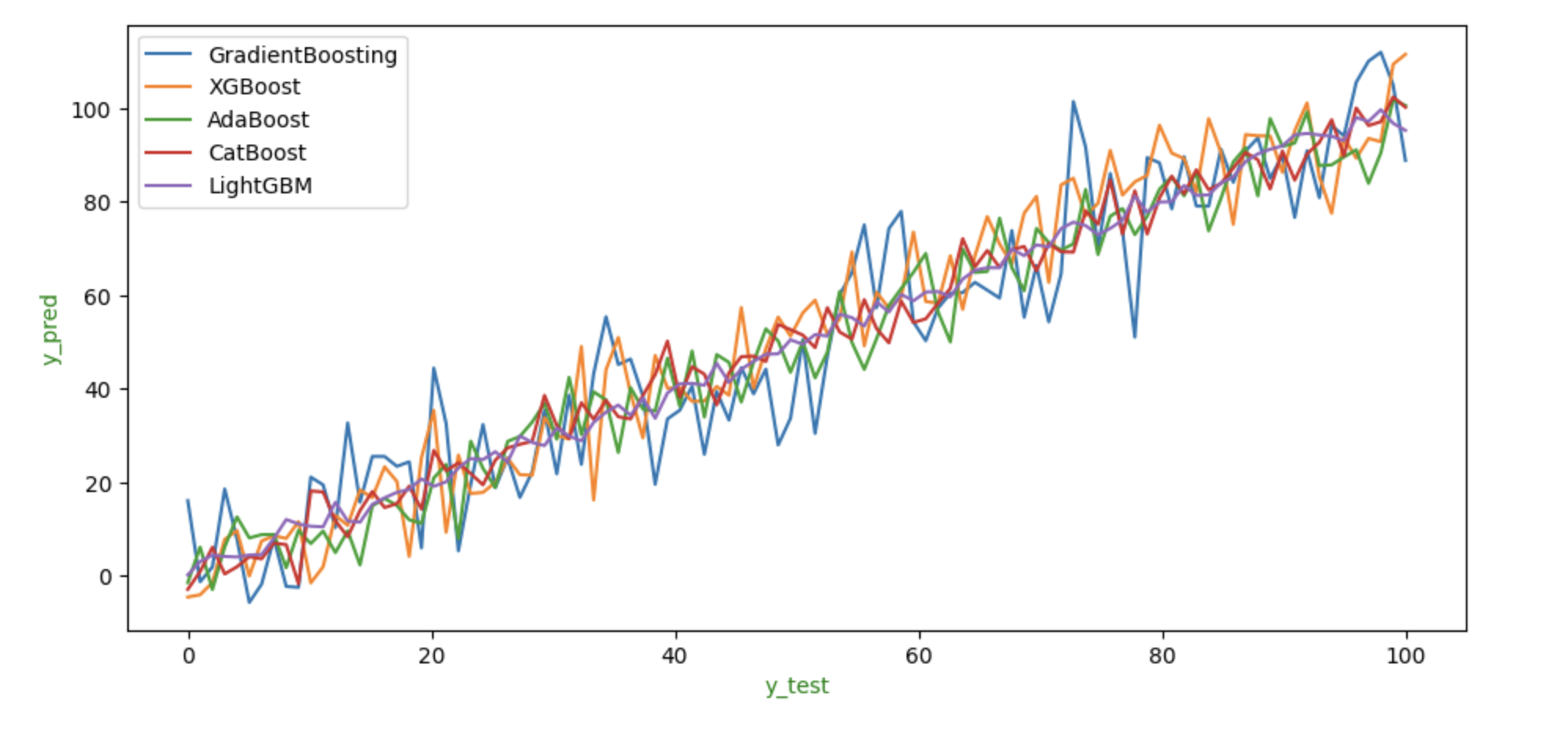
The image above shows the y_test and y_pred values expected by each method. We can see that LightGBM and CatBoost perform poorly when compared to other algorithms as they predict y_pred values that are much higher or lower than the other methods. As seen in the graph, XGBoost and GradientBoosting perform well all other algorithms on this data, with predictions that appear to be an average of all of them.

Difference between Different Boosting Algorithms

Here is the tabular difference between different boosting algorithms −

Feature	Gradient Boosting	LightGBM	XGBoost	CatBoost	AdaBoost
Year Introduced	Not specific	2017	2014	2017	1995
Handling Categorical Data	Needs extra steps like one-hot encoding	Needs extra steps	No special steps needed	Automatically handles it	No special steps needed
Speed/Scalability	Medium	Fast	Fast	Medium	Fast
Memory Usage	Medium	Low	Medium	High	Low
Regularization (Prevents Overfitting)	No	Yes	Yes	Yes	No
Parallel Processing (Runs Multiple Tasks at Once)	No	Yes	Yes	Yes	No
GPU Support (Can Use Graphics Card)	No	Yes	Yes	Yes	No
Feature Importance (Shows Which Features Matter)	Yes	Yes	Yes	Yes	Yes

Print Page