- LightGBM - Home
- LightGBM - Overview
- LightGBM - Architecture
- LightGBM - Installation
- LightGBM - Core Parameters
- LightGBM - Boosting Algorithms
- LightGBM - Tree Growth Strategy
- LightGBM - Dataset Structure
- LightGBM - Binary Classification
- LightGBM - Regression
- LightGBM - Ranking
- LightGBM - Implementation in Python
- LightGBM - Parameter Tuning
- LightGBM - Plotting Functionality
- LightGBM - Early Stopping Training
- LightGBM - Feature Interaction Constraints
- LightGBM vs Other Boosting Algorithms
- LightGBM Useful Resources
- LightGBM - Quick Guide
- LightGBM - Useful Resources
- LightGBM - Discussion
LightGBM - Implementation in Python
In this chapter, we will see the steps of developing a LightGBM model in Python. We will use Scikit-learn's load_breast_cancer dataset to build a binary classification model. The steps are as follows: load the data, prepare it for LightGBM, establish the parameters, train the model, make predictions, and evaluate the outcomes.
Implementation of LightGBM
So let us create a basic model using Python −
1. Load the Dataset
First, we load the dataset with Scikit-learn's load_breast_cancer method. This dataset contains features and labels for breast cancer classification.
from sklearn.datasets import load_breast_cancer

# Load dataset
data = load_breast_cancer()
X = data.data
y = data.target
2. Split the Data
The dataset is split into training and testing sets with Scikit-learn's train_test_split method. This allows us to train the model on one set of data and then evaluate its performance on another.
from sklearn.model_selection import train_test_split

# Split the data
X_train, X_test, y_train, y_test = train_test_split(X, y, test_size=0.2, random_state=42)
3. Prepare Data for LightGBM
Convert the training and testing data into LightGBM dataset format. This step optimizes the data format for LightGBM's training algorithms.
import lightgbm as lgb

# Convert the data to LightGBM dataset format
train_data = lgb.Dataset(X_train, label=y_train)
test_data = lgb.Dataset(X_test, label=y_test, reference=train_data)
4. Define Parameters
Set the parameters of the LightGBM model. These involve the objective function, evaluation metric, learning rate, leaf count, and maximum tree depth.
params = {
    'objective': 'binary',
    'metric': 'binary_logloss',
    'boosting_type': 'gbdt',
    'learning_rate': 0.1,
    # Increased from 31
    'num_leaves': 63,
    # Set to a positive value to limit depth
    'max_depth': 10
}
5. Train the Model
Train the LightGBM model using the training data. To prevent overfitting, we use early stopping, which means that training ends when no progress is seen on the validation set.
# Train the model with early stopping
lgb_model = lgb.train(
    params,
    train_data,
    num_boost_round=100,
    valid_sets=[test_data],
    # Use callback for early stopping
    callbacks=[lgb.early_stopping(stopping_rounds=10)]
)
Output
Here is the outcome of the above step −
[LightGBM] [Info] Number of positive: 286, number of negative: 169
[LightGBM] [Info] Auto-choosing col-wise multi-threading, the overhead of testing was 0.000734 seconds.
You can set `force_col_wise=true` to remove the overhead.
[LightGBM] [Info] Total Bins 4548
[LightGBM] [Info] Number of data points in the train set: 455, number of used features: 30
[LightGBM] [Info] [binary:BoostFromScore]: pavg=0.628571 -> initscore=0.526093
[LightGBM] [Info] Start training from score 0.526093
[LightGBM] [Warning] No further splits with positive gain, best gain: -inf
[LightGBM] [Warning] No further splits with positive gain, best gain: -inf
6. Make Predictions
Use the training model to predict the test data. We return the probability into binary outcomes.
# Predict on the test set
y_pred = lgb_model.predict(X_test)
y_pred_binary = [1 if x > 0.5 else 0 for x in y_pred]
7. Evaluate the Model
Calculate the accuracy score for the test set to evaluate the model's performance. This allows us to find out how well the model performs with previously unseen data.
from sklearn.metrics import accuracy_score

# Evaluate the model
accuracy = accuracy_score(y_test, y_pred_binary)
print(f"Accuracy: {accuracy:.2f}")
Output
Here is the accuracy of the above model −
Accuracy: 0.96
Exploratory Data Analysis (EDA) for the LightGBM Model
Exploratory Data Analysis (EDA) must be done before training and testing the LightGBM model in order to understand the dataset, identify patterns, and prepare it for modeling. EDA involves examining the dataset's structure, distributions, correlations, and potential issues.
Here are the steps on using EDA for the load_breast_cancer dataset −
1. Load and Inspect the Dataset
First we have to load the dataset and inspect its basic structure like the number of samples, features, and target variable.
import pandas as pd
from sklearn.datasets import load_breast_cancer

# Load dataset
data = load_breast_cancer()
df = pd.DataFrame(data.data, columns=data.feature_names)
df['target'] = data.target

# Inspect the dataset
print(df.head())
print(df.info())
print(df.describe())
Output
This will lead to the following outcome:
   mean radius  mean texture  mean perimeter  mean area  mean smoothness  \
0        17.99         10.38          122.80     1001.0          0.11840
1        20.57         17.77          132.90     1326.0          0.08474
2        19.69         21.25          130.00     1203.0          0.10960
3        11.42         20.38           77.58      386.1          0.14250
4        20.29         14.34          135.10     1297.0          0.10030

   mean compactness  mean concavity  mean concave points  mean symmetry  \
0           0.27760          0.3001              0.14710         0.2419
1           0.07864          0.0869              0.07017         0.1812
2           0.15990          0.1974              0.12790         0.2069
3           0.28390          0.2414              0.10520         0.2597
4           0.13280          0.1980              0.10430         0.1809

   mean fractal dimension  ...  worst texture  worst perimeter  worst area  \
0                 0.07871  ...          17.33           184.60      2019.0
1                 0.05667  ...          23.41           158.80      1956.0
2                 0.05999  ...          25.53           152.50      1709.0
3                 0.09744  ...          26.50            98.87       567.7
4                 0.05883  ...          16.67           152.20      1575.0

   worst smoothness  worst compactness  worst concavity  worst concave points  \
0            0.1622             0.6656           0.7119                0.2654
1            0.1238             0.1866           0.2416                0.1860
2            0.1444             0.4245           0.4504                0.2430
3            0.2098             0.8663           0.6869                0.2575
4            0.1374             0.2050           0.4000                0.1625

   worst symmetry  worst fractal dimension  target
0          0.4601                  0.11890       0
1          0.2750                  0.08902       0
2          0.3613                  0.08758       0
3          0.6638                  0.17300       0
4          0.2364                  0.07678       0
2. Check for Missing Values
Now let us see are there any missing values in the dataset.
# Check for missing values
print(df.isnull().sum())
Output
This will generate the below result:
mean radius                0
mean texture               0
mean perimeter             0
mean area                  0
mean smoothness            0
mean compactness           0
mean concavity             0
mean concave points        0
mean symmetry              0
mean fractal dimension     0
radius error               0
texture error              0
perimeter error            0
area error                 0
smoothness error           0
compactness error          0
concavity error            0
concave points error       0
symmetry error             0
fractal dimension error    0
worst radius               0
worst texture              0
worst perimeter            0
worst area                 0
worst smoothness           0
worst compactness          0
worst concavity            0
worst concave points       0
worst symmetry             0
worst fractal dimension    0
target                     0
dtype: int64
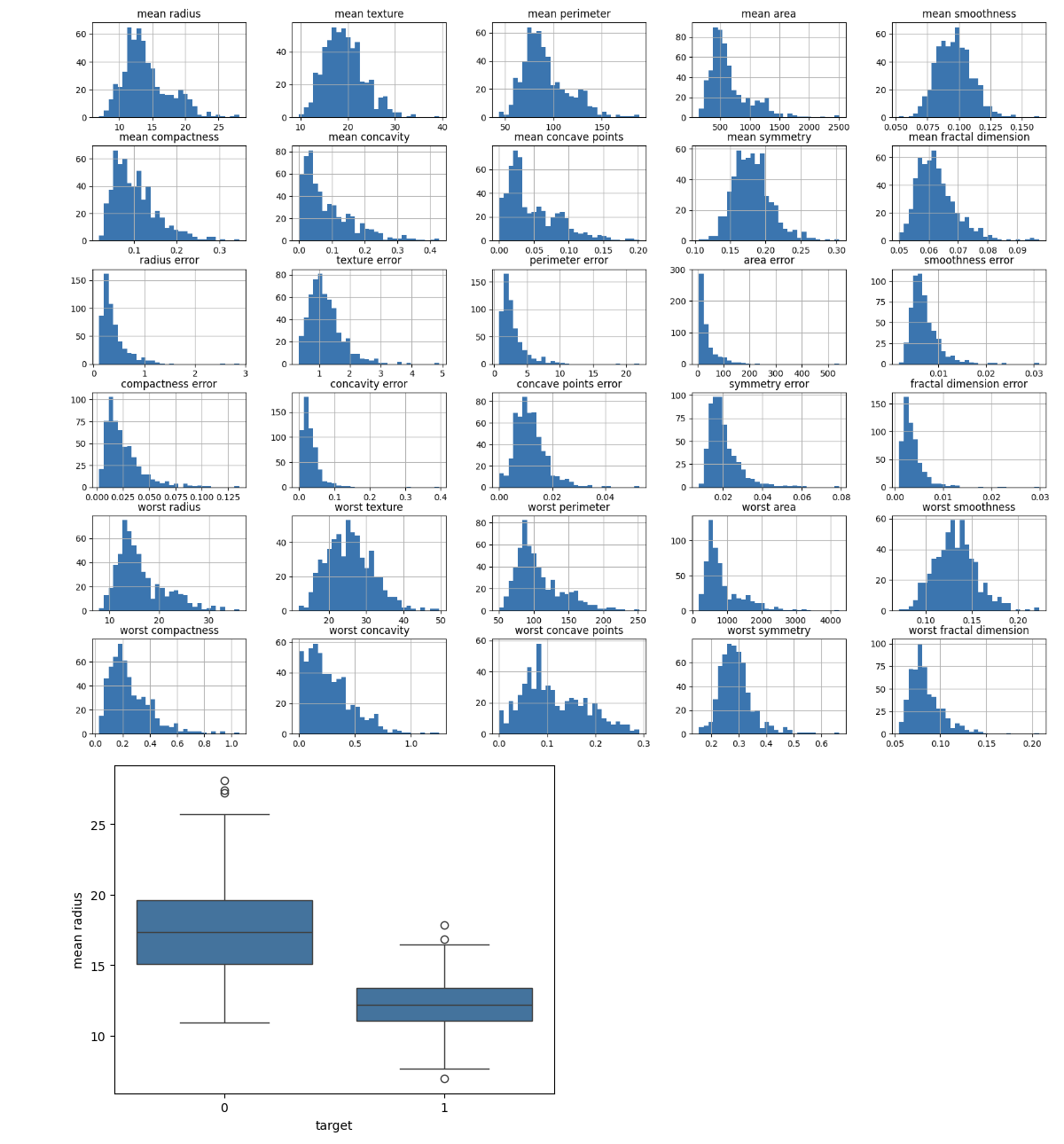
3. Feature Distributions
Determine the distribution of each feature. To understand more about the range and distribution of feature values, use histograms, box plots, or other visualizations.
import matplotlib.pyplot as plt
import seaborn as sns

# Plot histograms for each feature
df.iloc[:, :-1].hist(bins=30, figsize=(20, 15))
plt.show()

# Box plot for a selected feature
sns.boxplot(x='target', y='mean radius', data=df)
plt.show()
Output
This will create the below outcome:
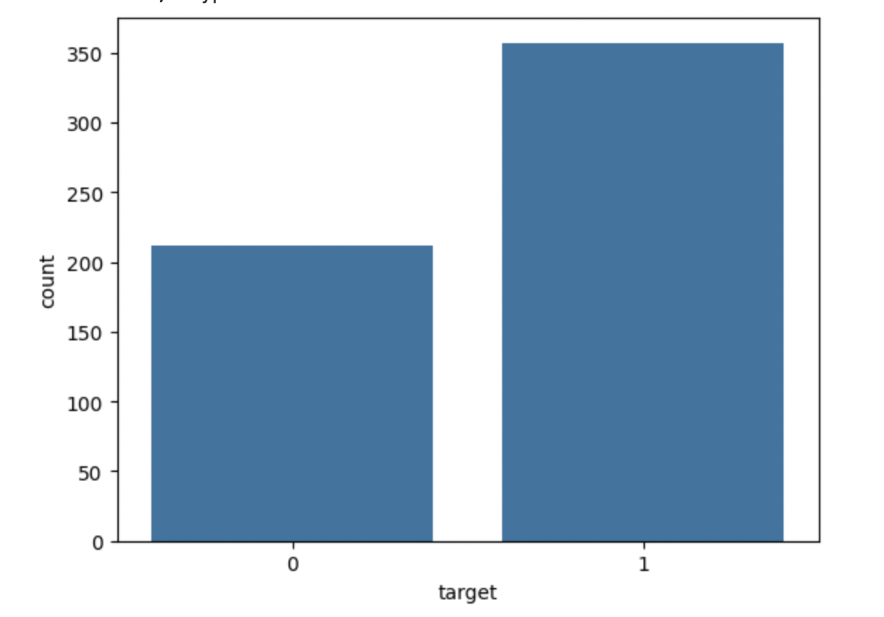
4. Analyze Class Distribution
Check the distribution of the target variable to find the class balance. This will allow you to identify if the dataset is imbalanced.
# Class distribution
print(df['target'].value_counts())
sns.countplot(x='target', data=df)
plt.show()
Output
This will show the below output −
target
1    357
0    212
Name: count, dtype: int64
Summary
Following these steps will allow you to create and test a LightGBM model for classification problems in Python. This technique can be modified for different datasets and problems by adjusting the parameters and preparation steps as needed.
