How to prevent top row from scrolling in Excel?

Introduction

Excel is a powerful spreadsheet application that can quickly manipulate and analyze large amounts of data. When working with massive datasets in Excel, it may be challenging to keep track of column names as you scroll down the screen. However, you may prevent rows or columns from disappearing while zooming in and out by freezing them in place using Excel's "Freeze Panes" feature. By following the steps outlined in this article, you may make Excel's top row permanent.

Why Does it Happen?

If you often lose sight of headers and labels as you navigate through big data sets, Excel's ability to freeze rows or columns is a useful tool to overcome this issue. This function was designed to help users and boost productivity by always displaying the most important information in the forefront.

As you scroll through a spreadsheet, Excel must relocate the visible portion of the page while keeping the headers or labels in their original positions. Because Excel scrolls the whole page by default, it might be difficult to locate certain rows and columns.

Users may get around this limitation by making advantage of Excel's Freeze Panes feature. Excel creates a separation between the frozen and scrollable parts of a spreadsheet when you do this. The frozen row or column is divided in two by drawing a boundary line below it or to its right. Excel locks in place the frozen rows or columns, keeping them in view while you navigate over the page.

When dealing with huge datasets, complicated spreadsheets, or when referencing specific information repeatedly, the option to freeze rows or columns is invaluable. You can quickly and simply grasp the facts without losing any context as you move across the page.

Follow these steps to set up this feature −

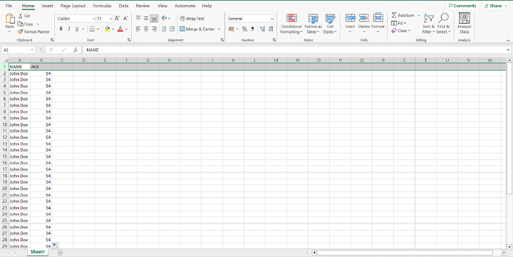
• Step 1 − Launch Excel and get into the data immediately.

• Step 2 − Freeze the row just underneath the one you want to save. Select Row 2 to end Row 1, for instance.

• Step 3 − select "View" from Excel's main menu at the top of the window.

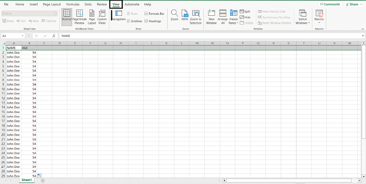
• Step 4 − Navigate to the "Window" sub-group under the "View" tab.

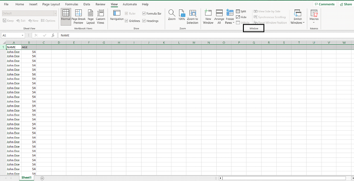
• Step 5 − Within the "Window" menu, select the "Freeze Panes" option.

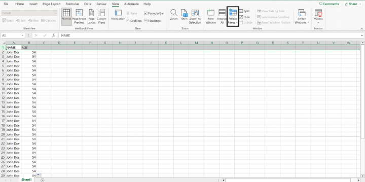
• Step 6 − A drop-down choice with different options will show up. Choose "Freeze Panes" from the list of options. Select Freeze Top Row option.

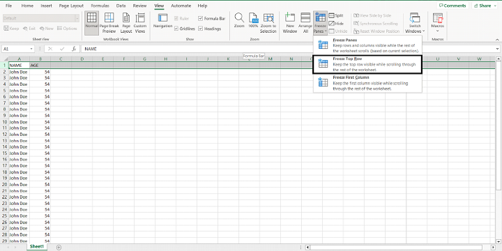
Doing so will fix the top row of your worksheet so it won't move as you navigate down the page. This makes it simple to scan the top row, whether for column labels or other data, from anywhere in the list.

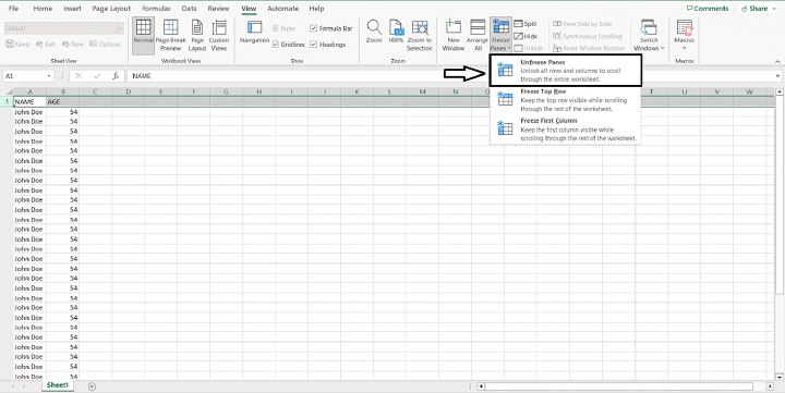
To restore normal scrolling after using the preceding procedures to freeze panes, just repeat those steps using the "Unfreeze Panes" option from the "Freeze Panes" menu.

Conclusion

Preventing the top row from scrolling in Excel is a valuable technique when working with large datasets that require constant reference to column headings or labels. By using the Freeze Panes feature, you can lock the top row in place, ensuring it remains visible and easily accessible regardless of how much you scroll through the spreadsheet. This feature enhances productivity and data analysis by keeping important information readily available.

Excel's Freeze Panes feature provides flexibility, allowing you to freeze multiple rows or columns as needed. By mastering this technique, you can effectively navigate and analyse data in Excel while maintaining a clear view of critical information.