How to lock specific column always visible in a sheet or across a workbook?

"Locking specific columns always visible in a sheet or across a workbook" in Excel refers to the ability to freeze or fix certain columns so that they remain visible on the screen even when scrolling horizontally through a large dataset or across different worksheets within a workbook.

By locking columns, you can ensure that specific information, such as headers or important data, remains in view regardless of how much you scroll horizontally or switch between different sections of a workbook. This feature is useful when working with wide datasets or when comparing information across multiple sheets within a workbook.

In this article, two examples are given. The first example is based on the use of available freeze pane options, as already specified.

Example 1: Lock columns are always visible in one sheet by the Freeze Panes option

Step 1

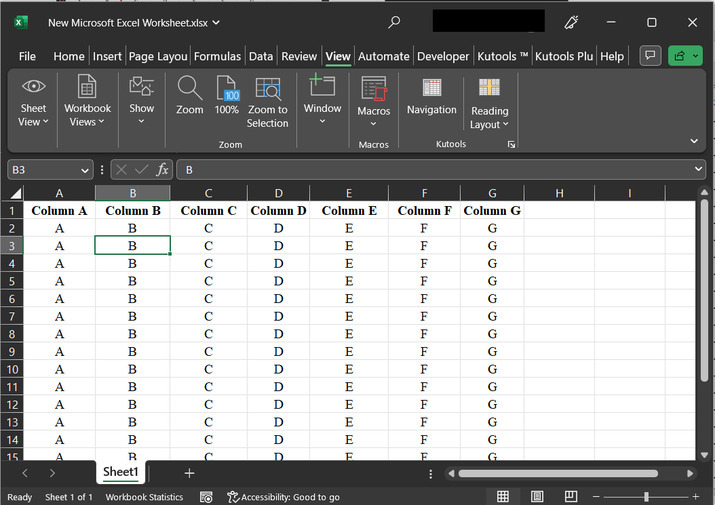
To understand the process of locking columns always visible from one side of the sheet, during sheet scrolling, firstly, Consider the below given Excel spreadsheet. In the below-given spreadsheet, will try to lock or freeze the first column.

Step 2

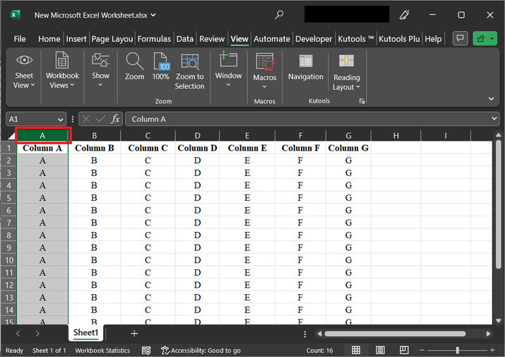
Select the first column. To select the first column, click on column header A. This will select the whole available column. Consider the below given snapshot for code, and understand that the selected column will be seen in highlighted grey color.

Step 3

Go to the “View” tab, and select the “Window” option. After that click on the “Freeze Panes”, and further select the option of “Freeze First Column”. This option will allow the user to freeze the first column of the provided Excel sheet.

Step 4

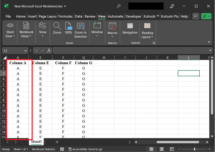
Consider the below provided Excel spreadsheet. Try to move the cursor forward to the A column. Users will observe that column A gets frozen while the other columns are moving frequently, without any issue.

Similarly, by utilizing the other two options as of freeze pane option, the user can easily freeze the rows and columns according to the requirement.

Example 2: Locking the same columns across multiple worksheets by using the Kutools for Excel

Step 1

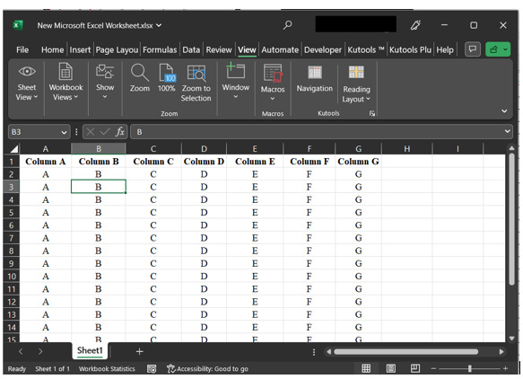
To understand the process of freezing the same set of rows and columns, across multiple sheets. Users need to use kutool option. Consider the same Excel sheet, as chosen for the above example. Consider the spreadsheet provided below −

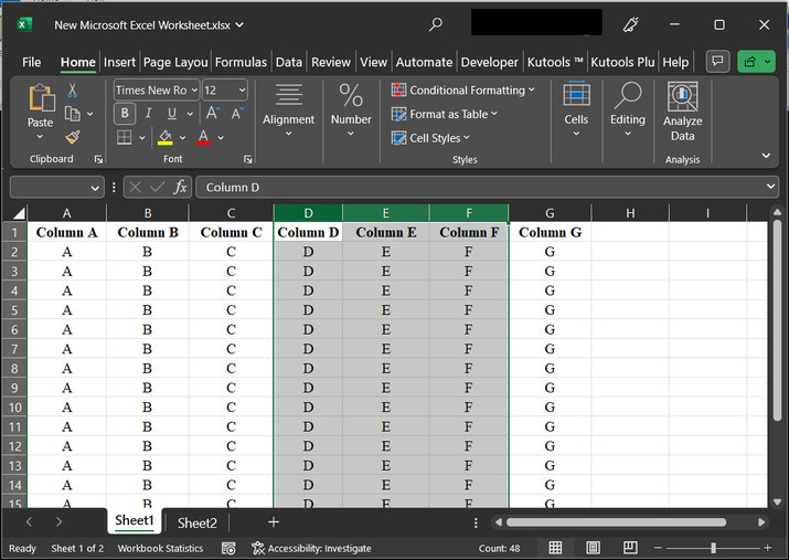
Step 2

In kutool user need to select the further columns to freeze the previous data. For example, if the user wants to freeze columns for A, B, and C. Then select the columns D, E, and F. to select the D, E, and F columns. First, click on the column header for D, and then press “Ctrl” key, along with that click on E and F column headers. To understand more precisely consider the below-given snapshot of the Excel worksheet.

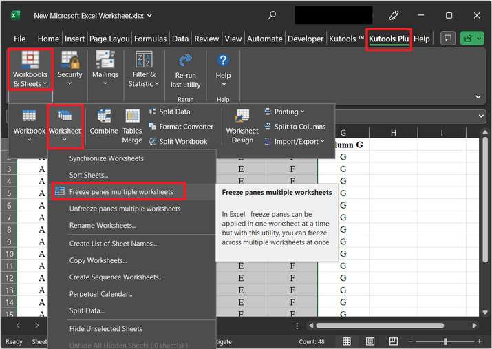
Step 3

Now, go to the “Kutool Plus” tab, and then click on the “Workbook & Sheets” tab, then click on the “Worksheet” option, further select the “Freeze panes multiple worksheets”, as depicted below −

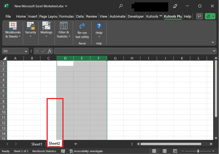
Step 4

Now, try to move the sheet by rolling the cursor further to the next column, and the user will observe that the column A, B, and C, will get fixed, while the rest columns are moving freely without any issue. Same with other sheets as well. That is in sheet 2, columns A, B, and C multiple columns will freeze automatically.

Conclusion

The two examples are illustrated in this article. The first example uses the concept of Freeze panes to lock a certain column. With the help of freeze pane options, either a specific row or column is locked as per user requirement. The second example uses the kutools to achieve the same task.