
Article Categories
- All Categories
-
 Data Structure
-
 Networking
-
 RDBMS
RDBMS
-
 Operating System
-
 Java
Java
-
 MS Excel
-
 iOS
iOS
-
 HTML
HTML
-
 CSS
CSS
-
 Android
-
 Python
-
 C Programming
-
 C++
C++
-
 C#
C#
-
 MongoDB
-
 MySQL
MySQL
-
 Javascript
-
 PHP
PHP
-
 Economics & Finance
How to Auto-Strikethrough Based on Cell Value in Excel?
Strikethrough is a type of data used in Excel to indicate that the data present in the cell is an error or that the event has been completed. The strikethrough is also used to represent that the event or process has successfully completed without any errors or mistakes.
Strikethrough is not a default font that we can use directly in Excel, but we can use it by applying an uncomplicated process. We can also add the strikethrough to the cells based on the cell value using conditional formatting. For example, we can add the strikethrough to cells with values greater than any specific value. Read this tutorial to learn how you can set Excel to auto-strikethrough based on cell value.
Auto-Strikethrough Based on Cell Value Using Conditional Formatting
Here we will use conditional formatting and select the strikethrough font under font. Let us see an uncomplicated process to understand how we can auto-add strikethrough based on cell value in Excel.
Step 1
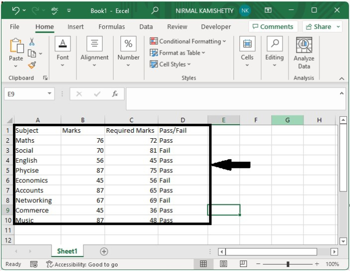
Let us consider an Excel sheet where the data present in the sheet is like the sheet shown in the below image.
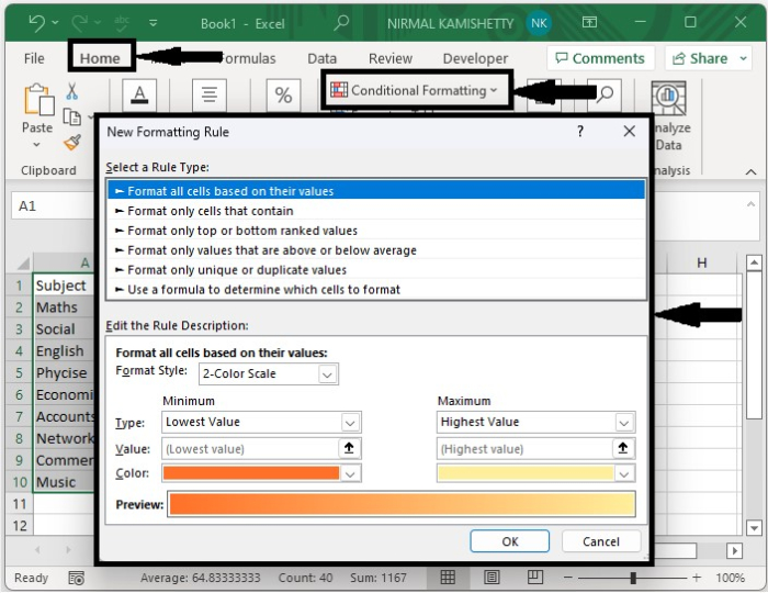
Now select the data, then click on conditional formatting under Home and select a new rule to open a pop-up as shown in the below image.
Step 2
Then, in the above pop-up, click on "use formula," enter the formula as =$D2="Fail," and then click on "format" to open a new pop-up. In the formula, D2 represents the cell address, and fail is the cell value you want to add a strikethrough based on.
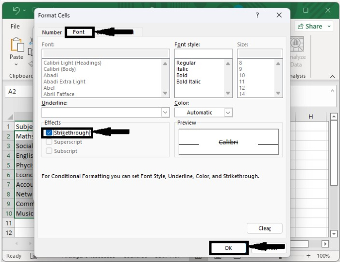
Again, in the new pop-up window, click on "Font" and select the checkbox beside the strikethrough, then click "OK" as shown in the below image.
Step 3
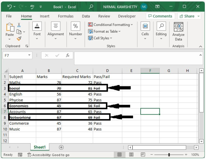
Finally, click OK, and our output will be successful, as shown in the image below.
Conclusion
In this tutorial, we used a simple example to demonstrate how you can automatically add strikethrough based on cell values in Excel.

8K+ Views
