How to highlight rows based on date in Google sheet?

In the article, the user will understand the process of highlighting the rows that contain date-type data within the Google sheet. There are several features available in the Google sheet such as conditional formatting, cell formatting, and many other features by using which users can perform the same required tasks. This article guide contains two examples, both the provided examples will allow the user to understand the way to handle the provided date data type effectively and efficiently. Both the provided examples are precise and accurate.

To highlight rows that contain date-type data in the Google sheet:

Example 1:

Step 1:

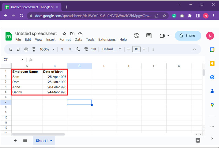
First, open the Google sheet and enter the below-given data into Google Sheets.

Step 2:

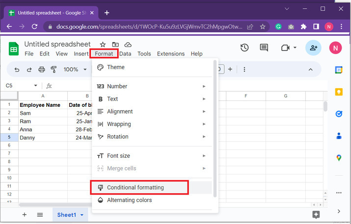
After that go to the format option and choose “Conditional formatting” as, depicted below:

Step 3:

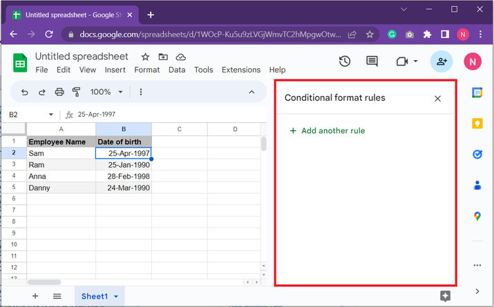
This will open the below-shown dialog box, on the right side of the Google sheet. Click on “Add another rule” under the “Conditional format rules” dialog box. This will open some new options.

Step 4:

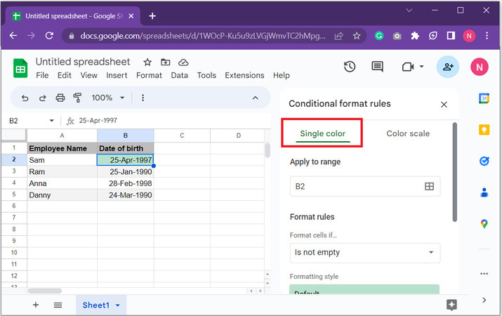
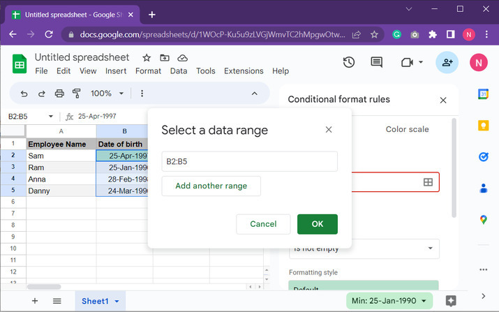
The appeared dialog box will open by default under the “Single color” tab. After that click on the “Apply to range” cell. Select the B column as it contains the date data that the user wants to highlight.

Step 5:

This will allow the sheet to automatically display the range as “B2:B5”. Simply click on “OK”.

Step 6:

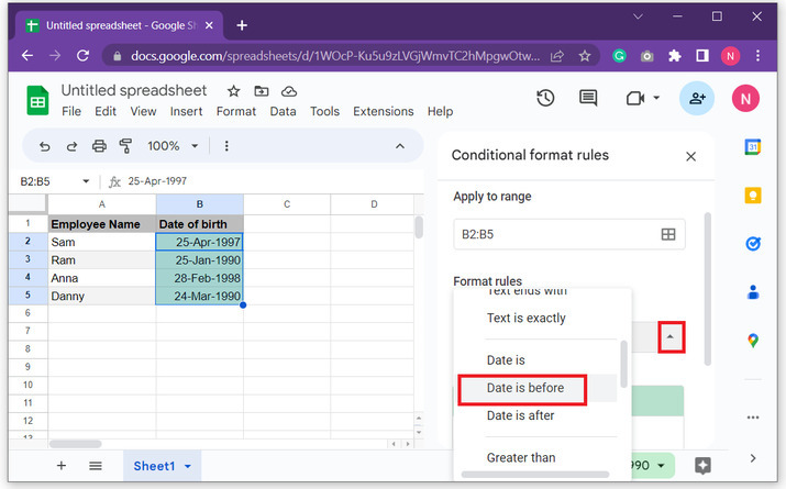
The selected data will appear on the right hand side. After that move to the next dialog box heading “format rules”, and click on the below highlighted drop-down button.

Step 7:

This will display multiple options in front of the user. For this example, select “Date is before” as highlighted in the below image:

Step 8:

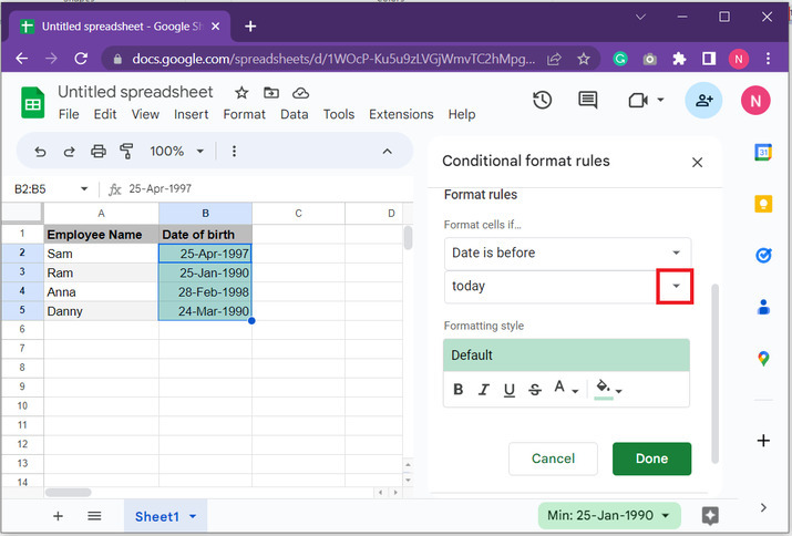
After that click on the next drop-down menu and select the option “today”. Finally click on the “Done” option.

Step 9:

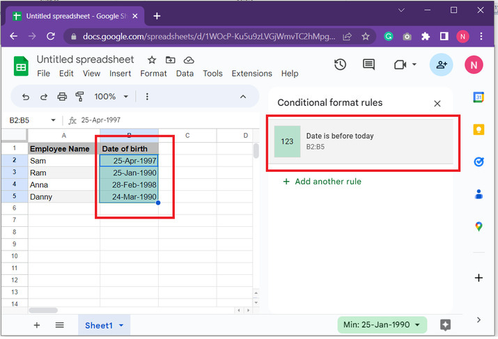
This will show the user created formatting rule under the “conditional format rules” pane, and will highlight all the dates that are of the date before today. As, this data contains date of birth of employees. Therefore, all the provided date of birth values are highlighted by the google sheet.

Example 2:

Step 1:

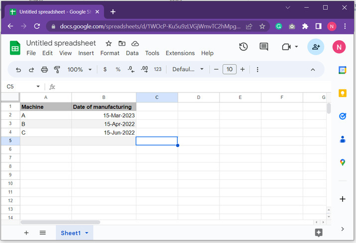
First, open the Google sheet and enter the below-given data to google sheet.

Step 2:

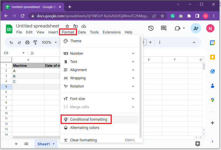
To apply the conditional formatting rule, go to the “Format” tab and “Conditional formatting” as shown in below image:

Step 3:

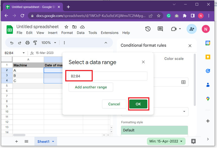
The new dialog box would appear named Select a data Range. After that select the range “B2:B4”, by either using the mouse or by manually entering the data, into the sheet. Click on the provided button “OK”.

Step 4:

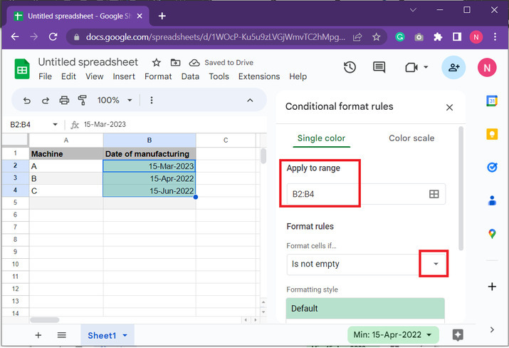
After that move to the “format rules” section, and click on the first drop-down menu. Consider below given highlighted arrow for reference:

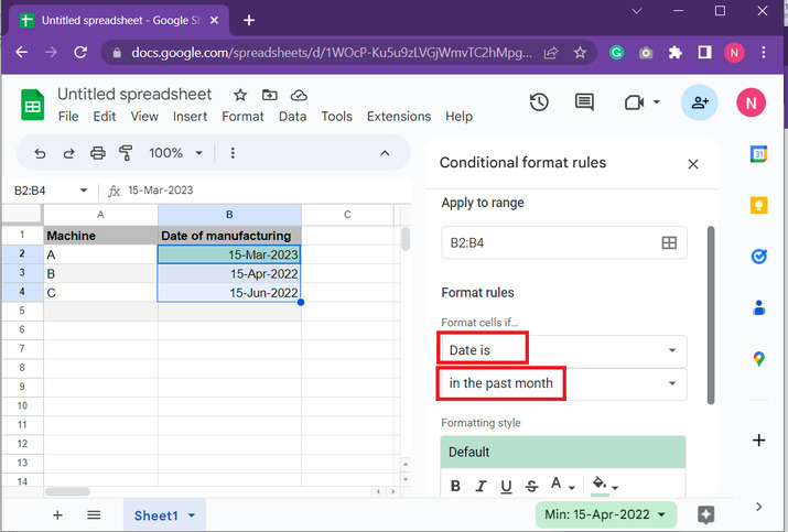
Step 5:

In the first drop-down menu choose “Date is”, and in the next available drop-down menu, select “in the past month” option. Consider the below given image for proper reference:

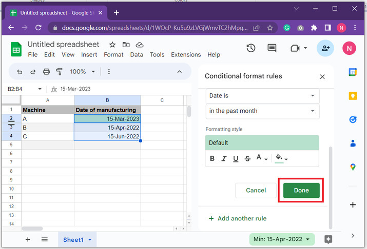
Step 6:

Finally, scroll down the section, and click on the “Done” button.

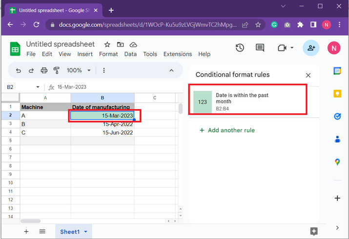
Step 7:

This will display the above-developed formatting rule, in the right hand side pane. The table will highlight the row that will fulfill the specified condition. In this case, a user wants to highlight the row values that contain the date from the previous month. This will help to take account of the machine manufactured last month.

Conclusion:

This tutorial allow user to understand the way to handle rows that contains date type data. First example allow user to highlight the date before the current day date. In more clear ways, example 1 will highlight the date before today. Now, let’s discuss about the second example, second example will highlight the dates for previous month.