How To Do Sensitivity Analysis With Data Table In Excel?

Sensitivity analysis is a powerful tool that helps decision−makers assess the impact of changing input values on the outcome of a model or calculation. By creating a data table in Excel, you can quickly and easily analyse various scenarios and determine the sensitivity of your results to different variables. In this tutorial, we will guide you through the process of setting up and using a data table in Excel to conduct sensitivity analysis. Whether you are a business professional, a financial analyst, or a student working on a project, this tutorial will provide you with the knowledge and skills to perform sensitivity analysis efficiently.

Throughout the tutorial, we will provide step−by−step instructions accompanied by screenshots to ensure a clear understanding of the process. We will also discuss best practices, tips, and common pitfalls to help you avoid any potential errors. By the end of this tutorial, you will have the skills to perform sensitivity analysis with a data table in Excel, empowering you to make informed decisions based on various scenarios and inputs. So, let's dive in and unlock the power of sensitivity analysis in Excel!

Do Sensitivity Analysis With Data Table

Here we will first make changes to the data, then create a sensitivity analysis table, and finally use the what−if analysis to complete the task. So let us see a simple process to learn how you can do sensitivity analysis with a data table in Excel.

Step 1

Consider an Excel sheet. The data in the sheet is similar to the below image.

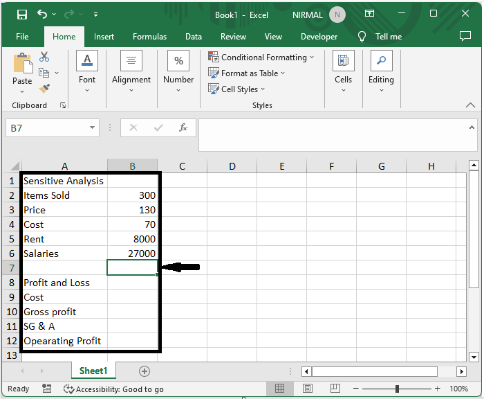
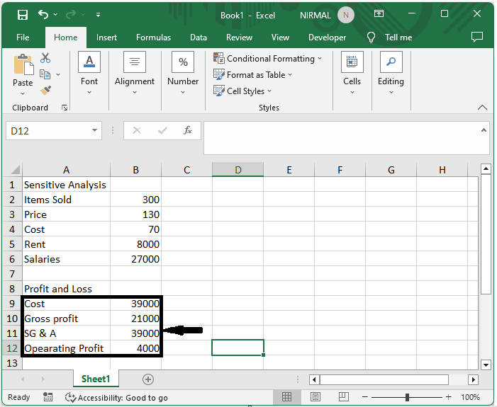
First, enter the formula in the cells B9, B10, B11, and B12 as =B2*B3, =B4*B2, =B9−B8, and =B11−B5−B6, respectively.

Empty cells > Formulas > Enter.

Step 2

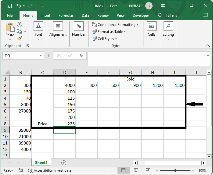
Then Prepare the sensitivity analysis table as below screenshot shown −

In Range E2:I2, please type the sales volumes from 300 to 1500

In Range D3:D8, please type the prices from 100 to 225

In the Cell D2, please type the formula =B12

Step 3

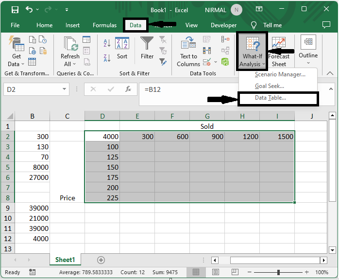
Then select the range of cells D2:I8, click on data, and select the data table under What−If Analysis.

Select cells > Data > What−If Analysis > Data Table.

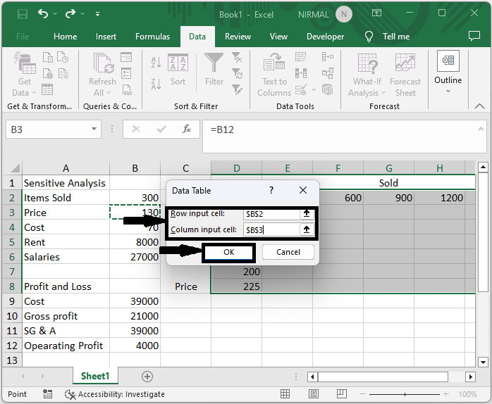
Step 4

Then in the pop−up, set the row input cell as cell $B$2 and the column input cell as $B$3, and click OK to complete the task.

Conclusion

In this tutorial, we have used a simple example to demonstrate how you can do sensitivity analysis with a data table in Excel to highlight a particular set of data.