
Article Categories
- All Categories
-
 Data Structure
-
 Networking
-
 RDBMS
RDBMS
-
 Operating System
-
 Java
Java
-
 MS Excel
-
 iOS
iOS
-
 HTML
HTML
-
 CSS
CSS
-
 Android
-
 Python
-
 C Programming
-
 C++
C++
-
 C#
C#
-
 MongoDB
-
 MySQL
MySQL
-
 Javascript
-
 PHP
PHP
-
 Economics & Finance
How To Display / Show Auto Filter Criteria In Excel?
With the help of Excel's auto filters, you can swiftly sort and filter data in a spreadsheet. However, occasionally being able to see the filtering criteria that have been used on a specific column can be helpful. You can better comprehend and examine your data with the use of this information. This article will show you how to simply check and review the filtering requirements by displaying or showing the auto filter criteria in Excel. This course will provide you the knowledge and skills to fully utilise Excel's filtering features, regardless of your level of Excel proficiency. In order to successfully display or exhibit auto filter criteria in Excel, let's get started.
Display / Show Auto Filter Criteria
Here we will create a custom formula using the VBA application and use it to complete the task. So let us see a simple process to know how you can display or show auto?filter criteria in Excel.
Step 1
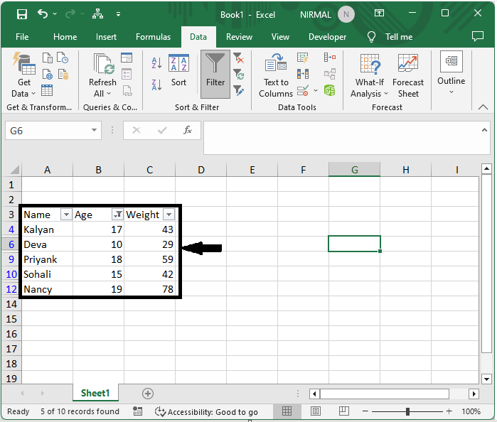
Consider an Excel sheet where the data in the sheet is similar to the below image.
First, right?click on the sheet name and select "View Code" to open the VBA application. Then click on "Insert" and select "Module".
Right click > View code > Insert > Module.
Step 2
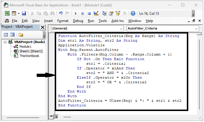
Then copy the below code into the text box and close the VBA, similar to the below image.
Copy > Alt + Q.
Code
Function AutoFilter_Criteria(Rng As Range) As String
Dim str1 As String, str2 As String
Application.Volatile
With Rng.Parent.AutoFilter
   With .Filters(Rng.Column - .Range.Column + 1)
      If Not .On Then Exit Function
         str1 = .Criteria1
      If .Operator = xlAnd Then
         str2 = " AND " & .Criteria2
      ElseIf .Operator = xlOr Then
         str2 = " OR " & .Criteria2
      End If
   End With
End With
AutoFilter_Criteria = UCase(Rng) & ": " & str1 & str2
End Function
Step 3
Then click on an empty cell, in our case, cell A1, and enter the formula as
=AutoFilter_Criteria(A4) then drag the auto?fill handle towards the right to complete the task.
Empty cell > Formula > Enter > Drag.

Conclusion
In this tutorial, we have used a simple example to demonstrate how you can display or show auto?filter criteria in Excel to highlight a particular set of data.

858 Views
