
Article Categories
- All Categories
-
 Data Structure
-
 Networking
-
 RDBMS
RDBMS
-
 Operating System
-
 Java
Java
-
 MS Excel
-
 iOS
iOS
-
 HTML
HTML
-
 CSS
CSS
-
 Android
-
 Python
-
 C Programming
-
 C++
C++
-
 C#
C#
-
 MongoDB
-
 MySQL
MySQL
-
 Javascript
-
 PHP
PHP
-
 Economics & Finance
How to Auto-Fit Column Width in Excel?
Adjusting the width of each column in Excel is one of the most frequently used processes. When we use formats like date, we can see that the width of the cell is automatically fitted, but this does not always happen. When the width of the cells is not enough to display the data, then a series of "#" symbols will be displayed in the cell. This problem can be solved using the auto-fit function.
Read this tutorial to learn how you can autofit column width in Excel.
AutoFit Column Width in Excel
Here, we'll use three simple shortcuts to complete our task. Let us see a simple process to understand how we can automatically adjust the column width in Excel. To complete the process, we will use the shortcut keys.
Step 1
Consider an Excel sheet with data that is clumsy and similar to the data shown in the image below.
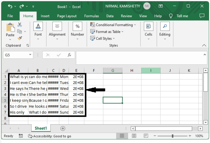
As we can see, the fact that the data represented in the sheet is not clear and impossible to understand can be solved just by adjusting the width of each column. We can do it manually, but generally we don?t use it. In general, it will be done using the shortcut keys. We will be using the commands that are combined with the ALT button.
Step 2
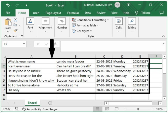
Now select the range of cells you want to adjust and click the commands ALT+O, ALT+C, and ALT+A sequentially, and the widths of the column will be adjusted as shown in the below image.
Note ? Make sure that you don?t release the ALT button while giving the commands, that is, click O, C, and A separately with a single click of the ALT button.
Conclusion
In this tutorial, we used a simple example to demonstrate how we can auto-fit column width in Excel to highlight a particular set of data.

777 Views
