
Article Categories
- All Categories
-
 Data Structure
-
 Networking
-
 RDBMS
RDBMS
-
 Operating System
-
 Java
Java
-
 MS Excel
-
 iOS
iOS
-
 HTML
HTML
-
 CSS
CSS
-
 Android
-
 Python
-
 C Programming
-
 C++
C++
-
 C#
C#
-
 MongoDB
-
 MySQL
MySQL
-
 Javascript
-
 PHP
PHP
-
 Economics & Finance
How to Average Cells Based on Multiple Criteria in Excel?
In Excel, we average the value based on no conditions. Our requirements are only a list of numbers, and we can calculate the average easily. But have you ever tried to calculate the average based on conditions? We can do this by using the formulas. This tutorial will help you understand how we can average cells based on multiple criteria in Excel. In this tutorial, I will demonstrate two methods for calculating the average in Excel: one using a single criterion and another based on multiple criteria.
Average Cells Based on Single Criteria
Here we will get the average by matching the cell value. Let us see a straightforward process to see how we can average cells based on single criteria, and we can complete this by using the formulas.
Let us consider an Excel sheet where the data is like the data shown in the below image.
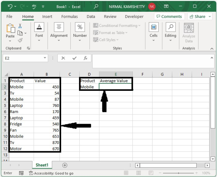
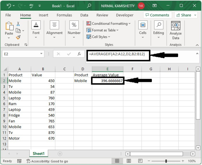
Now, in the empty cell, enter the formula =AVERAGEIF(A2:A12,D2, B2:B12) and press enter to get the result shown in the image below. In the formula, A2:A12 is the range of products, B2:12 is the range of values, and D2 is the address of the cell where we have the criteria.
Average Cells Based on Multiple Criteria
In this section, we will calculate the average based on cell value. Let us see an effortless process to see how we can average cells based on multiple criteria, and we can complete this by using the formulas.
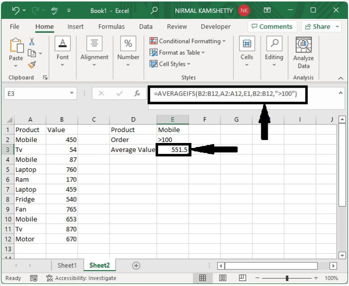
Let us consider the same data that we used in the above example. The other criteria we are using in the example is that the value should be greater than one hundred.

Now click on an empty cell and enter the formula as
=AVERAGEIFS(B2:B12,A2:A12,E1,B2:B12,">100") then click OK to get the result shown in the below image.
Conclusion
In this tutorial, we used a simple example to demonstrate how we can average cells based on multiple criteria in Excel.

751 Views
