
Article Categories
- All Categories
-
 Data Structure
-
 Networking
-
 RDBMS
RDBMS
-
 Operating System
-
 Java
Java
-
 MS Excel
-
 iOS
iOS
-
 HTML
HTML
-
 CSS
CSS
-
 Android
-
 Python
-
 C Programming
-
 C++
C++
-
 C#
C#
-
 MongoDB
-
 MySQL
MySQL
-
 Javascript
-
 PHP
PHP
-
 Economics & Finance
How To Display Negative Numbers In Brackets In Excel?
Excel is a strong tool for calculations and data analysis, and it provides a number of formatting options to improve the visual representation of your data. Negative numbers are frequently formatted using brackets, which can make it simpler to identify them from positive values.
In this tutorial, we'll look at how to set up Excel to automatically display negative values in brackets step?by?step. We'll go over several approaches, such as leveraging Excel's built?in number formatting features and developing unique formatting rules. By the end of this article, you will be able to present negative values in brackets with ease, giving your Excel spreadsheets a polished appearance. Let's get started and discover how to display negative values in Excel brackets!
Display Negative Numbers In Brackets In Excel
Here we will format the range of cells to complete the task. So let us see a simple process to learn how you can display negative numbers in brackets in Excel.
Step 1
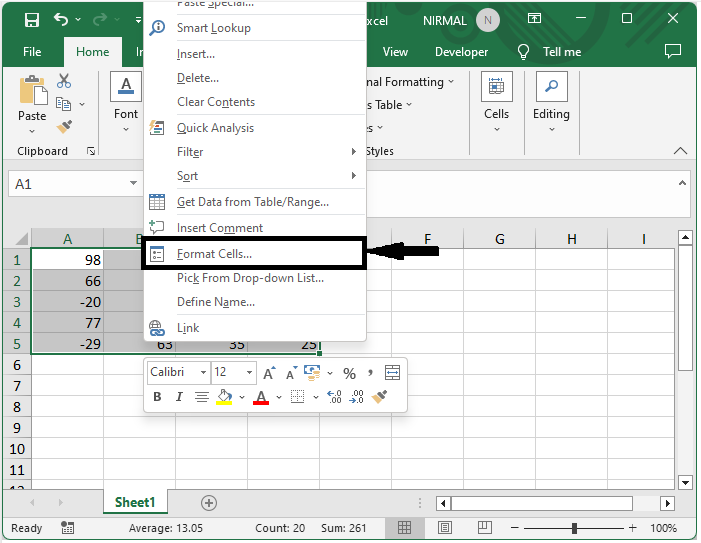
Consider an Excel sheet where you have a list of positive and negative numbers.
First, select the range of cells, then right?click and select format cells.
Select cells > Right click > Format cells.
Step 2
Then form the list click on custom and enter type as 0.00;[Red](0.00) and click ok to complete the task. This will display negative numbers in brackets.
Number > Custom > Type > Ok.
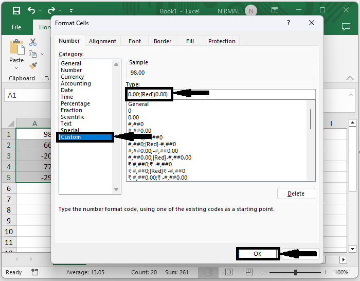
Then you can see that all the negative numbers will be displayed inside the brackets, and then the minus symbol will be removed.

This is how you can display negative numbers in brackets in Excel.
Conclusion
In this tutorial, we have used a simple example to demonstrate how you can display negative numbers in brackets in Excel to highlight a particular set of data.

51K+ Views
