

- Excel - Home
- Excel - Getting Started
- Excel - Explore Window
- Excel - Backstage
- Excel - Entering Values
- Excel - Move Around
- Excel - Save Workbook
- Excel - Create Worksheet
- Excel - Copy Worksheet
- Excel - Hiding Worksheet
- Excel - Delete Worksheet
- Excel - Close Workbook
- Excel - Open Workbook
- Excel - Merge Workbooks
- Excel - File Password
- Excel - File Share
- Excel - Emoji & Symbols
- Excel - Context Help
- Excel - Insert Data
- Excel - Select Data
- Excel - Delete Data
- Excel - Move Data
- Excel - Rows & Columns
- Excel - Copy & Paste
- Excel - Find & Replace
- Excel - Spell Check
- Excel - Zoom In-Out
- Excel - Special Symbols
- Excel - Insert Comments
- Excel - Add Text Box
- Excel - Shapes
- Excel - 3D Models
- Excel - CheckBox
- Excel - Add Sketch
- Excel - Scan Documents
- Excel - Auto Fill
- Excel - SmartArt
- Excel - Insert WordArt
- Excel - Undo Changes
- Formatting Cells
- Excel - Setting Cell Type
- Excel - Move or Copy Cells
- Excel - Add Cells
- Excel - Delete Cells
- Excel - Setting Fonts
- Excel - Text Decoration
- Excel - Rotate Cells
- Excel - Setting Colors
- Excel - Text Alignments
- Excel - Merge & Wrap
- Excel - Borders and Shades
- Excel - Apply Formatting
- Formatting Worksheets
- Excel - Sheet Options
- Excel - Adjust Margins
- Excel - Page Orientation
- Excel - Header and Footer
- Excel - Insert Page Breaks
- Excel - Set Background
- Excel - Freeze Panes
- Excel - Conditional Format
- Excel - Highlight Cell Rules
- Excel - Top/Bottom Rules
- Excel - Data Bars
- Excel - Color Scales
- Excel - Icon Sets
- Excel - Clear Rules
- Excel - Manage Rules
- Working with Formula
- Excel - Formulas
- Excel - Creating Formulas
- Excel - Copying Formulas
- Excel - Formula Reference
- Excel - Relative References
- Excel - Absolute References
- Excel - Arithmetic Operators
- Excel - Parentheses
- Excel - Using Functions
- Excel - Builtin Functions
- Excel Formatting
- Excel - Formatting
- Excel - Format Painter
- Excel - Format Fonts
- Excel - Format Borders
- Excel - Format Numbers
- Excel - Format Grids
- Excel - Format Settings
- Advanced Operations
- Excel - Data Filtering
- Excel - Data Sorting
- Excel - Using Ranges
- Excel - Data Validation
- Excel - Using Styles
- Excel - Using Themes
- Excel - Using Templates
- Excel - Using Macros
- Excel - Adding Graphics
- Excel - Cross Referencing
- Excel - Printing Worksheets
- Excel - Email Workbooks
- Excel- Translate Worksheet
- Excel - Workbook Security
- Excel - Data Tables
- Excel - Pivot Tables
- Excel - Simple Charts
- Excel - Pivot Charts
- Excel - Sparklines
- Excel - Ads-ins
- Excel - Protection and Security
- Excel - Formula Auditing
- Excel - Remove Duplicates
- Excel - Services
- Excel Useful Resources
- Excel - Keyboard Shortcuts
- Excel - Quick Guide
- Excel - Functions
- Excel - Useful Resources
- Excel - Discussion
Excel - Format Number
MS Excel has a plethora of formatting options and inbuilt statistical functions. You can benefit from these formatting options to make the worksheet consistent and in a readable form. General is a standard category of number formatting in Excel.
For example, you have downloaded the sales.xls worksheet from the web, and its two columns, sales contact number and invoice dates, are in different formats and not in readable form. To eliminate these formatting challenges, you can get the tremendous benefits of the number formatting presented in the Format Cells dialog box.
Excel Number Formatting
Excel number formatting can be done in two ways −
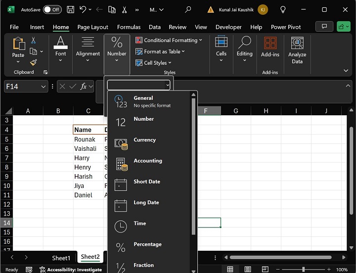
1. Go to the Home tab and select the "Number Format" button from the Number group, where the list of the categories is showcased in the drop-down menu. The Accounting Number Format, Percent Style, Comma Style, Increase Decimal, and Decrease decimal are available in the Number group.
2. Use the keyword shortcut "ctrl+1" to open the Format cells and select the Number tab to facilitate Excel number formatting.
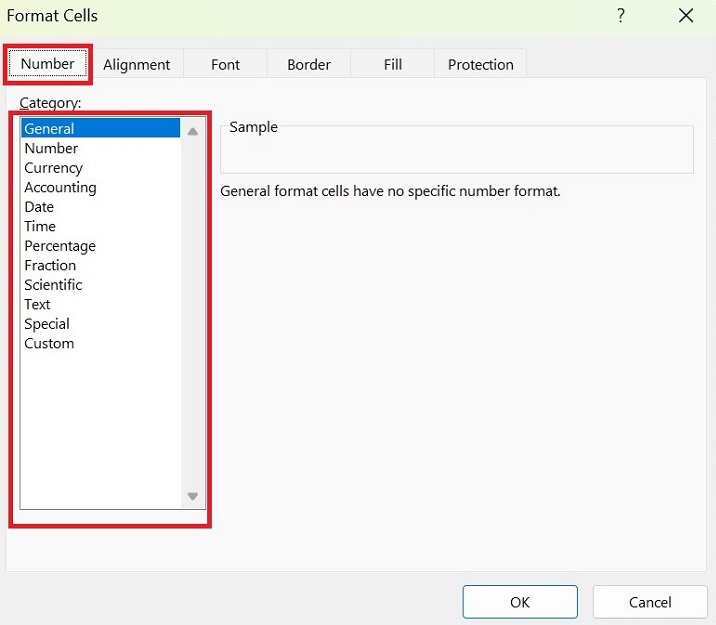
Categories of the Excel Number Formatting are listed below −
- General
- Number
- Currency
- Accounting
- Date
- Time
- Percentage
- Fraction
- Scientific
- Text
- Special
- Custom
Example of Format Number in Excel
Lets get started with a few exciting examples
Example 1: How to apply phone number formatting in excel?
Step 1 − Consider the sample datasets consisting of two columns: Sales Executive and Phone Numbers.
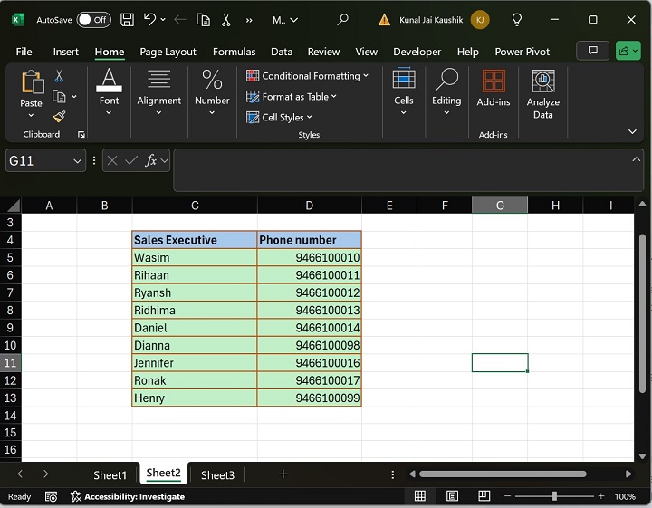
Step 2 − Select the range D5:D13 to format the phone numbers in Microsoft Excel. Use the "ctrl+1" keyboard shortcut to open the "Format Cells" dialog box.
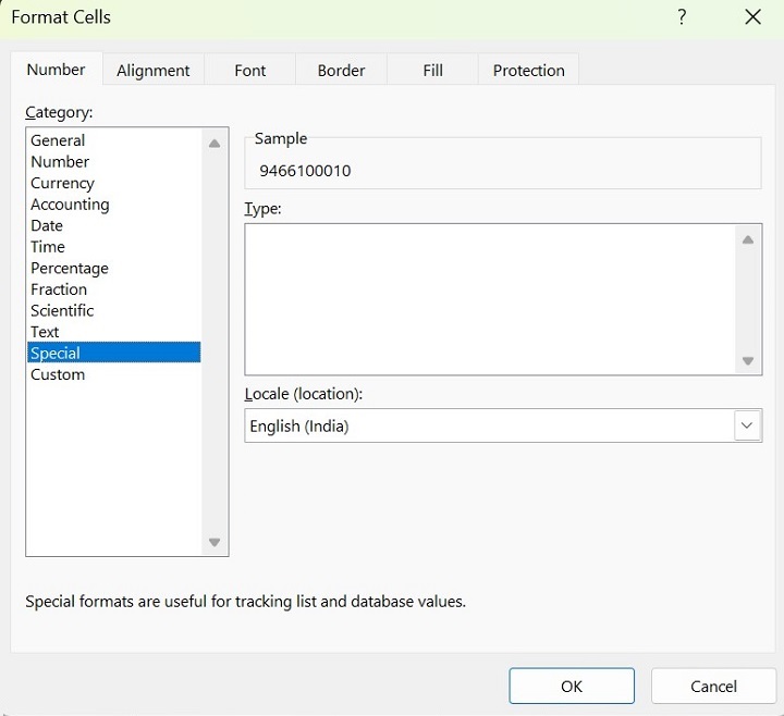
Step 3 − You can select the "Special" option from the Category box and select the phone number in the Type list. However, the Type list is empty in a few Excel versions.
Note − If you are using Excel 365, then the Type list is not populated.
In that case, you can select the "Custom" option from the Category − box and write the "[<=9999999]###-####;(###) ###-####" in the Type: box and click the OK button.
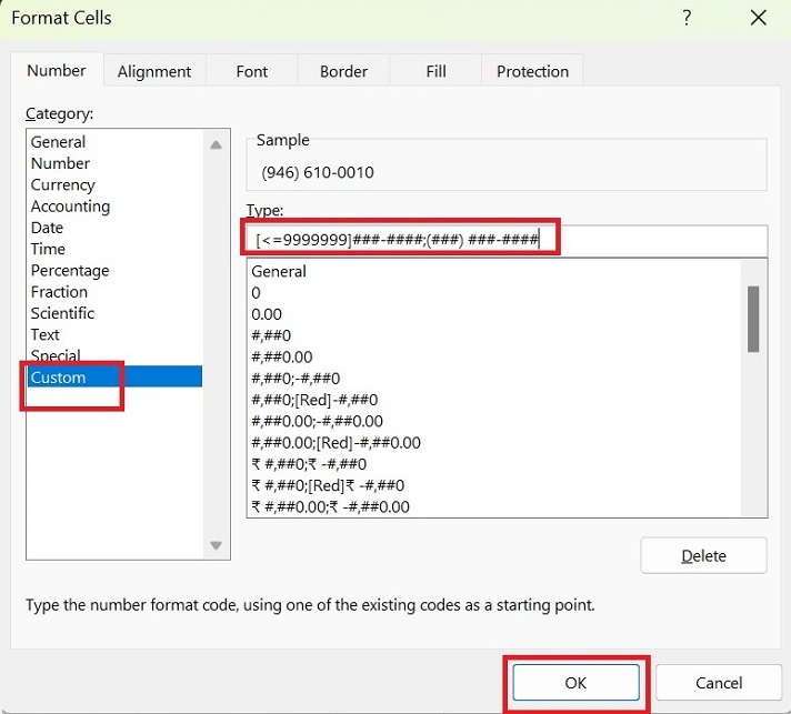
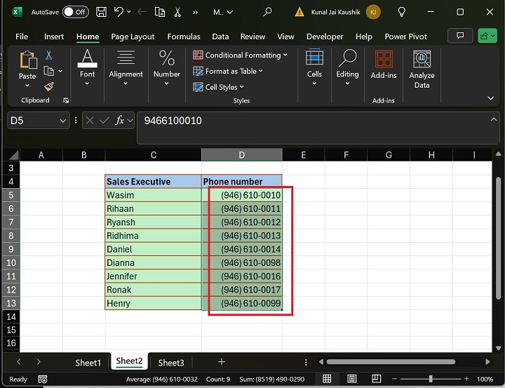
Hence, we have transformed the general Numbers in the phone number formatting in Microsoft Excel.
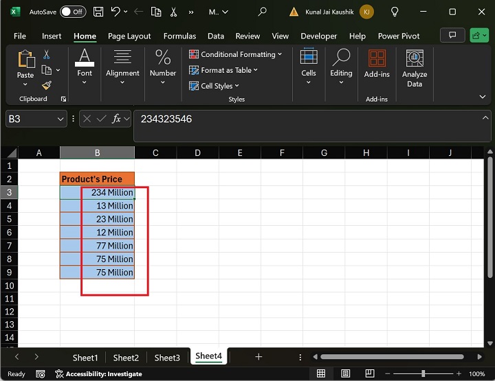
Example 2: Excel Numbers Formatting for Millions
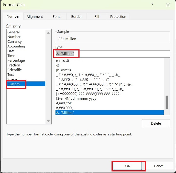
Step 1 − Lets say you have a list of products' prices specified in the general number. Select the cell range B3:B8 and press "Ctrl+1" to open the Format Cells dialog box.

In the Format Cells dialog box, select the Custom option from the Category section, write the #, "Million" in the Type Box, and press the OK button.
Example 3: How to use Scientific Notation number formatting in Excel?
Various steps are given below to use the Scientific Notation −
1. First, select the range of B3:B10 that specifies the product's price in the Manufacturing company.

2. After that, switch to the Home tab. Choose the Scientific option from the "Number Format" drop-down menu under the Number group.
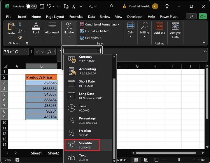
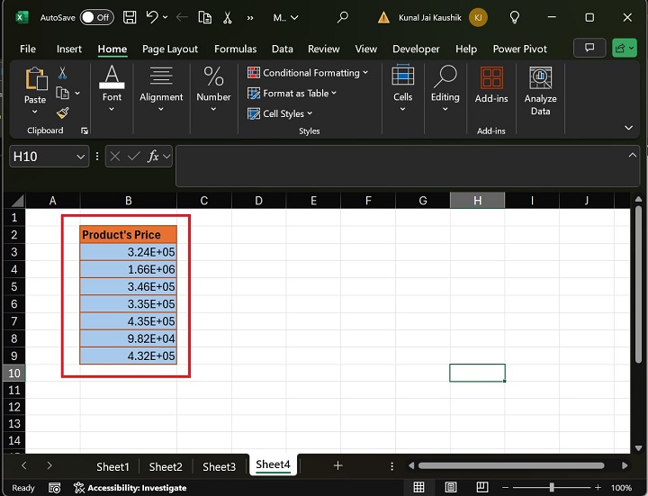
3. Once you click the "Scientific" option, the specified cell range values have been converted to Scientific Notation. For example, after selecting the Scientific Notation, the 323546 integer is transformed to 3.24E+05, equivalent to the 3.24*10^7. The original values will remain on the back end.
Example 4: Date Formatting in Microsoft Excel
Beginners usually encounter challenges in entering Dates in the specified format. Lets say you entered the date 23/09/2023 in the cell. But after entering this date, it is displayed in the numbers.
In this example, Henry entered a few dates in the B column. However, the general numbers are shown despite the respective dates.
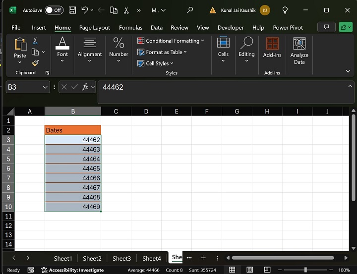
Henry selected the range B3:B10 and quickly pressed the "ctrl+1" keyboard shortcut to open the "Format Cells" dialog box. Furthermore, you can select the "Date" from the Category section and select the "14 March 2012" option from the Type section. Finally, press the Enter tab.
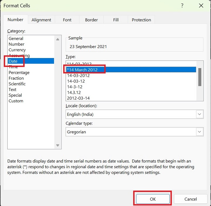
Therefore, the Date Formatting in Excel has transformed all the numbers into Dates.