
Article Categories
- All Categories
-
 Data Structure
-
 Networking
-
 RDBMS
RDBMS
-
 Operating System
-
 Java
Java
-
 MS Excel
-
 iOS
iOS
-
 HTML
HTML
-
 CSS
CSS
-
 Android
-
 Python
-
 C Programming
-
 C++
C++
-
 C#
C#
-
 MongoDB
-
 MySQL
MySQL
-
 Javascript
-
 PHP
PHP
-
 Economics & Finance
How to create normal quantile-quantile plot for a logarithmic model in R?
How to create normal quantile-quantile plot for a logarithmic model in R?
A logarithmic model is the type of model in which we take the log of the dependent variable and then create the linear model in R. If we want to create the normal quantile-quantile plot for a logarithmic model then plot function can be used with the model object name and which = 2 argument must be introduced to get the desired plot.
Example1
> x1<-rnorm(100,5,1)
> x1
Output
[1]  4.735737 3.631521 5.522580 5.538314 5.580952 4.341072 4.736899 2.455681
[9]  4.042295 5.534034 4.717607 6.146558 4.466849 5.444437 5.390151 4.491595
[17] 4.227620 4.223362 5.452378 5.690660 5.321716 5.269895 2.810042 4.295378
[25] 5.767740 3.939896 6.213647 4.608487 5.094318 4.621997 4.801568 6.329819
[33] 4.339835 3.172058 6.031193 5.123346 5.673534 5.668435 5.754537 4.164556
[41] 6.630504 5.209786 7.171595 4.713524 4.382267 5.204943 5.895252 4.413933
[49] 5.491437 3.806081 6.283097 4.892824 3.698107 4.758340 3.612643 4.670258
[57] 5.376201 6.440996 3.589660 4.990421 6.649452 5.549918 4.224869 5.604002
[65] 4.667142 5.522634 4.820425 4.278682 4.611169 3.801012 4.774964 4.678297
[73] 4.087518 5.705981 5.812739 4.585449 3.328274 3.626282 4.637604 3.707011
[81] 5.661713 4.671823 6.033384 3.553500 3.945178 3.065177 4.260533 5.226990
[89] 4.852304 4.995663 5.229401 6.588605 5.375225 6.089018 4.199044 6.520236
[97] 5.569930 7.400434 6.291279 4.593149
Example
> y1<-rpois(100,10)
> y1
Output
[1] 10 13 10 11 12 10 7 10 15 6 6 7 8 11 14 16 7 11 14 11 7 7 9 7 7
[26] 13 8 11 12 14 13 8 12 6 9 15 10 8 9 12 11 12 9 10 12 15 11 14 12 13
[51] 8 8 19 10 7 9 9 16 13 8 8 6 9 11 11 18 11 12 12 15 7 12 10 8 10
[76] 10 14 11 5 9 6 11 13 8 9 10 6 6 13 12 14 12 9 11 11 8 9 12 13 5
> Model1<-lm(log(y1)~x1)
> summary(Model1)
Call:
lm(formula = log(y1) ~ x1)
Residuals:
Min 1Q Median 3Q Max
-0.69827 -0.19657 0.01667 0.19465 0.61978
Coefficients:
Estimate Std. Error t value Pr(>|t|)
(Intercept) 2.39474 0.15197 15.758 <2e-16 ***
x1 -0.01895 0.03011 -0.629 0.531
---
Signif. codes: 0 ‘***’ 0.001 ‘**’ 0.01 ‘*’ 0.05 ‘.’ 0.1 ‘ ’ 1
Residual standard error: 0.2895 on 98 degrees of freedom
Multiple R-squared: 0.004024, Adjusted R-squared: -0.006139
F-statistic: 0.3959 on 1 and 98 DF, p-value: 0.5307
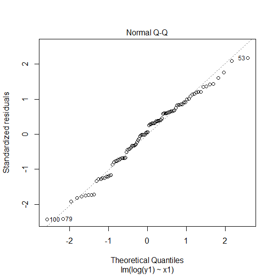
Creating the normal quantile-quantile plot:
> plot(Model1,which=2)
Output:
Example2
> x2<-rpois(100,5)
> x2
Output
[1]  3 7 13 4 6 2 4 3 2 7 4 6 3 11 6 5 5 6 6 2 3 7 8 3 1
[26] 8 5 2 2 3 7 6 7 4 7 2 4 3 4 2 5 2 4 5 3 5 8 5 3 3
[51] 6 2 8 3 4 7 3 5 5 3 7 4 7 6 6 6 10 5 4 3 5 7 3 3 5
[76] 4 9 3 7 8 7 2 6 5 7 5 6 6 5 3 9 9 5 4 2 5 5 5 6 4
Example2
> y2<-rpois(100,12)
> y2
Output
[1]  16 8 10 12 11 11 6 15 3 12 8 11 9 12 8 18 7 13 10 17 15 17 15 10 11
[26] 12 16 12 17 13 11 17 16 14 15 10 12 9 10 14 9 6 12 17 14 9 10 9 13 5
[51] 16 12 17 11 10 12 13 18 12 14 19 9 14 11 14 12 6 7 6 16 9 10 11 15 10
[76] 11 8 13 7 16 19 18 8 13 15 11 7 12 7 9 9 14 14 13 15 10 14 11 13 11
> Model2<-lm(log(y2)~x2)
> summary(Model2)
Call:
lm(formula = log(y2) ~ x2)
Residuals:
Min 1Q Median 3Q Max
-1.31858 -0.17210 0.04939 0.21912 0.50892
Coefficients:
Estimate Std. Error t value Pr(>|t|)
(Intercept) 2.409861 0.081191 29.681 <2e-16 ***
x2 0.003665 0.014863 0.247 0.806
---
Signif. codes: 0 ‘***’ 0.001 ‘**’ 0.01 ‘*’ 0.05 ‘.’ 0.1 ‘ ’ 1
Residual standard error: 0.327 on 98 degrees of freedom
Multiple R-squared: 0.00062, Adjusted R-squared: -0.009578
F-statistic: 0.0608 on 1 and 98 DF, p-value: 0.8057
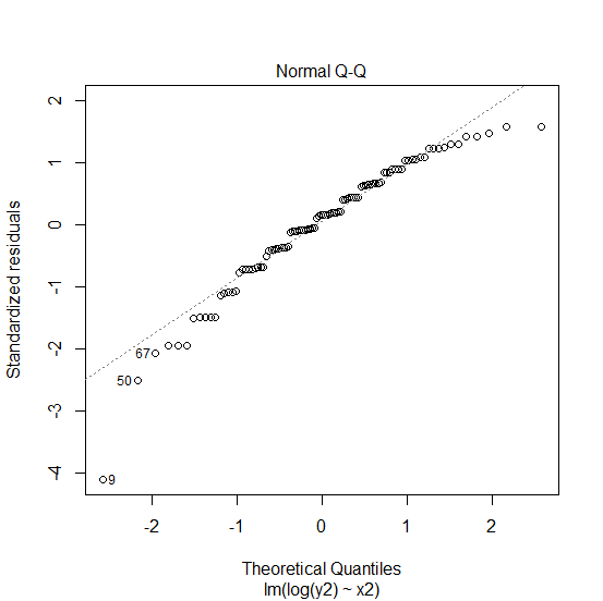
Creating the normal quantile-quantile plot:
> plot(Model2,which=2)
Output:

349 Views
