
Article Categories
- All Categories
-
 Data Structure
-
 Networking
-
 RDBMS
RDBMS
-
 Operating System
-
 Java
Java
-
 MS Excel
-
 iOS
iOS
-
 HTML
HTML
-
 CSS
CSS
-
 Android
-
 Python
-
 C Programming
-
 C++
C++
-
 C#
C#
-
 MongoDB
-
 MySQL
MySQL
-
 Javascript
-
 PHP
PHP
-
 Economics & Finance
How To Create Dynamic Hyperlink Based On Specific Cell Value In Excel?
Excel is a powerful tool for organizing and analyzing data, and one of its most useful features is the ability to create dynamic hyperlinks. With dynamic hyperlinks, you can link to other cells or worksheets within your workbook, or to external resources such as websites or files. The best part is that the link destination can change based on the value of a specific cell, which makes it a useful tool for creating interactive reports or dashboards. In this tutorial, we will show you how to create dynamic hyperlinks in Excel based on specific cell values, so you can take your data analysis to the next level. Whether you're a beginner or an experienced Excel user, this tutorial will help you unlock the full potential of dynamic hyperlinks in your workbooks.
Create Dynamic Hyperlink Based On Specific Cell Value
Here, we will first create a data validation list and then use the hyperlink formula to complete the task. So let us see a simple process to know how you can create dynamic hyperlinks based on a specific cell value in Excel.
Step 1
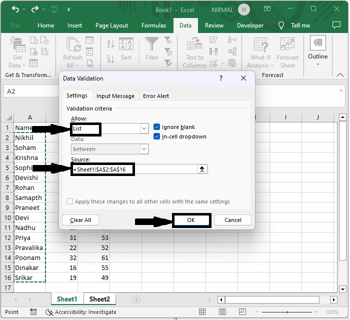
Consider an Excel sheet where the data is similar to the below image.

First, select an empty cell, then click on data and select data validation. Then set the allow to list option, selected the source as a range of cells, and clicked OK.
Empty cell > Data > Data validation > Allow > Source > Ok.
Step 2
Now click on the empty cell beside the data validation list and enter the formula as =HYPERLINK("#"&CELL("address",INDEX(Sheet1!A2:A16,MATCH(A2,Sheet1!A2:A16,0))),"Jump to the data cell") and click enter to complete our task.

Conclusion
In this tutorial, we have used a simple example to demonstrate how you can create dynamic hyperlinks based on specific cell values in Excel to highlight a particular set of data.

16K+ Views
