
Article Categories
- All Categories
-
 Data Structure
-
 Networking
-
 RDBMS
RDBMS
-
 Operating System
-
 Java
Java
-
 MS Excel
-
 iOS
iOS
-
 HTML
HTML
-
 CSS
CSS
-
 Android
-
 Python
-
 C Programming
-
 C++
C++
-
 C#
C#
-
 MongoDB
-
 MySQL
MySQL
-
 Javascript
-
 PHP
PHP
-
 Economics & Finance
How to Count/Sum Cells by Colors with Conditional Formatting in Excel?
You can visually highlight cells using the strong tool of conditional formatting based on certain criteria, such as colour. Utilising this function allows you to calculate depending on the colours assigned to certain cells, as well as highlight key data points. We will walk you through the process of counting or adding cells based on their colours step by step in this lesson. Whether you're a novice or a seasoned Excel user, this article will show you how to fully utilise conditional formatting to effectively analyse and work with data.
Make sure you have a fundamental understanding of Excel and the formatting choices available before we start. This guide will presume that you are already familiar with the basic ideas behind spreadsheets and are comfortable using Excel's user interface. So let's get started and see how to use conditional formatting in Excel to count or sum cells according on their colour!
Count/Sum Cells by Colours with Conditional Formatting
Here, we will first create a VBA module and then run it to complete the task. So let us see a simple process to know how you can count or sum cells by colour with conditional formatting in Excel.
Step 1
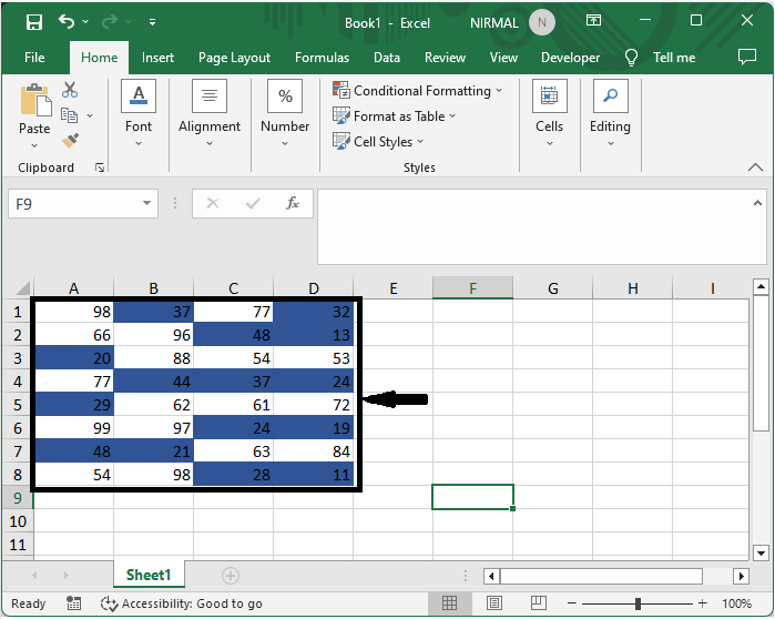
Consider an Excel sheet where you have a range of cells with different fill colours , similar to the below image.
First, right-click on the sheet name and select View Code to open the VBA application.
Right click > View code.
Step 2
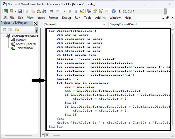
Then click on Insert, select Module, and copy the below code into the text box.
Insert > Module > Copy.
Code
Sub DisplayFormatCount()
	Dim Rng As Range
	Dim CountRange As Range
	Dim ColorRange As Range
	Dim xBackColor As Long
	Dim xFontColor As Long
	On Error Resume Next
	xTitleId       = "Count Cell Colour"
	Set CountRange = Application.Selection
	Set CountRange = Application.InputBox("Count Range :", xTitleId, CountRange.Address, Type: = 8)
	Set ColorRange = Application.InputBox("Color Range(single cell):", xTitleId, Type: = 8)
	Set ColorRange = ColorRange.Range("A1")
	xReturn        = 0
	For Each Rng In CountRange
		qqq           = Rng.Value
		xxx           = Rng.DisplayFormat.Interior.Color
		If Rng.DisplayFormat.Interior.Color = ColorRange.DisplayFormat.Interior.Color Then
         xBackColor   = xBackColor + 1
		End If
		If Rng.DisplayFormat.Font.Color = ColorRange.DisplayFormat.Font.Color Then
			xFontColor = xFontColor + 1
		End If
	Next
	MsgBox "BackColor is " & xBackColor & Chr(10) & "FontColor is " & xFontColor
End Sub
Step 3
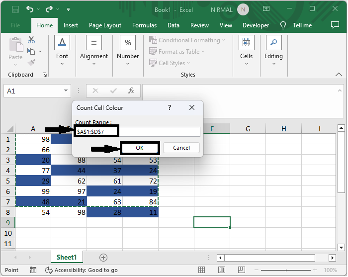
Now click F5 to run the module, select the range of cells, and click Ok.
Step 4
Then select the single cell and click OK.

Then you can see that result will be pop up. This is how you can count by colours with conditional formatting.
Conclusion
In this tutorial, we have used a simple example to demonstrate how you can count or sum cells by colour with conditional formatting in Excel to highlight a particular set of data.

1K+ Views
