
Article Categories
- All Categories
-
 Data Structure
-
 Networking
-
 RDBMS
RDBMS
-
 Operating System
-
 Java
Java
-
 MS Excel
-
 iOS
iOS
-
 HTML
HTML
-
 CSS
CSS
-
 Android
-
 Python
-
 C Programming
-
 C++
C++
-
 C#
C#
-
 MongoDB
-
 MySQL
MySQL
-
 Javascript
-
 PHP
PHP
-
 Economics & Finance
How to Average Cells Ignoring Error Values in Excel?
You could have always tried to average cells where there are no error values. But have you ever faced a situation where you wanted to average the range of data but were not able to do that because of the presence of error values? This tutorial will help you understand how we can average cells while ignoring error values in Excel. The error can be of any type; for example, it can be a division error or a reference error. We can complete processes directly in Excel using the program's formulas. We can use the array formulas to complete the process.
Average Cells Ignoring Error Values
Here we will use the formula, which is the combination of AVERAGE and ISERROR. Let us see an uncomplicated process to see how we can average cells while ignoring error values in Excel. We can complete the process by using the array formulas in Excel.
Step 1
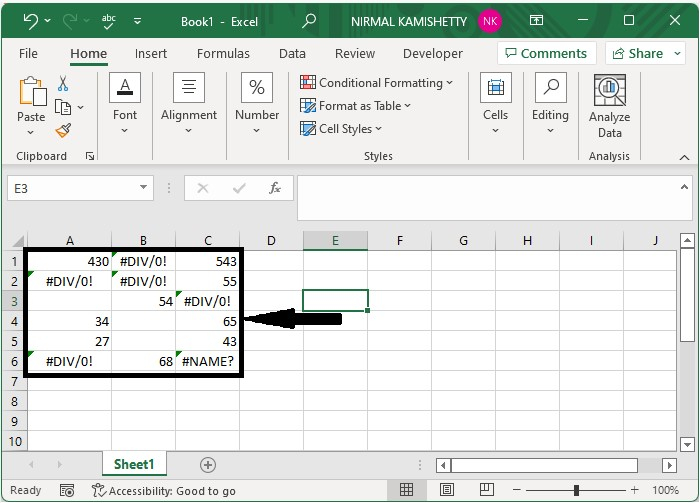
Let us consider an Excel sheet where the data is like the data shown in the below image.
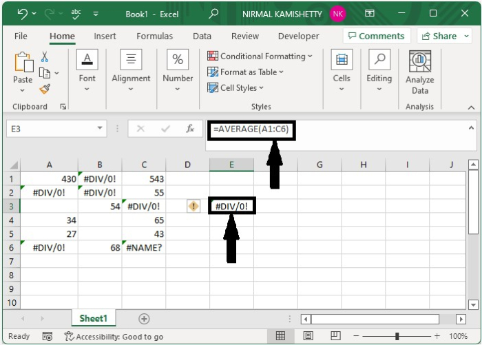
We now try to get the average value directly by clicking on an empty cell, typing the formula =AVERAGE(A1:C6), and pressing Enter. The result will be an error, as shown in the below image, because of the presence of error values in the range.
Step 2
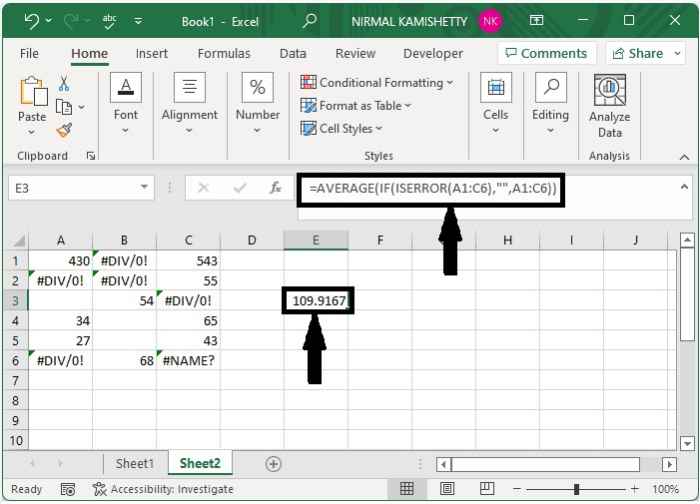
To get the average value while ignoring the error values, click on an empty cell and enter the formula =AVERAGE(IF(ISERROR(A1:C6),"",A1:C6) in the cell and press Enter, as shown in the image below. In the formula, A1:C6 is the range where we want to find the average value. The error value will be ignored in the selected range because of the keyword we used, "ISERROR."
Conclusion
In this tutorial, we used a simple example to demonstrate how we can average cells in Excel while ignoring error values.

6K+ Views
