How to Assign a Value or Category Based on a Number Range in Excel?

Assume we have a problem where we want to give students grades based on their grades, such as if they got 90 to 100 percent, give them an "O", and if they got less than 50 percent, give them "L" grades. If we try to do this manually, it could be a very time-consuming process. We can solve this problem by using the many formulas supported by Excel at a very rapid rate.

Read this tutorial to understand how you can assign a value based on a number in Excel. This process can be completed using two methods: the first is using the IF and AND functions, and the other is using the VLOOKUP function.

Assigning a Value or Category Based on a Number Range Using IF and the AND Functions

Here, we will first get the first result using the formula, then fill in all the results using the auto-fill handle. Let us see a simple process to assign a value or category based on a number range using IF and the AND function in Excel.

Step 1

Assume we have an excel sheet with data similar to the data shown in the image below. 

Now, in cell C2, click on an empty cell and enter the formula as follows: 

=IF(AND(B2>=0,B2<=200),"D",IF(AND(B2>200,B2<=300),"C",IF(AND(B2>300,B2<=500),"B",IF(AND(B2>500),"A",0)))) and click on Enter to get the first result, as shown in the below image.

Step 2

We got the first result successfully, and we can get all the other results just by dragging from the first result until all the results are successfully printed, and our final result will be similar to the below image.

Assigning a Value or Category Based on a Number Range Using VLOOKUP Function

Here we will create the grading list separately and use the VLOOKUP function to get the results. Let us see a simple process to assign values based on a number range using the VLOOKUP function.

Step 1

Let us consider that we have an excel sheet where the data in the sheet contains a list of marks and grading similar to the below image.

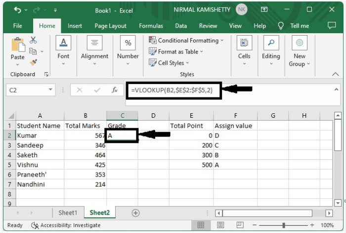
To get the first result, click on cell C2 and enter the formula =VLOOKUP(B2,$E$2:$F$5,2) in the formula box, then press Enter.

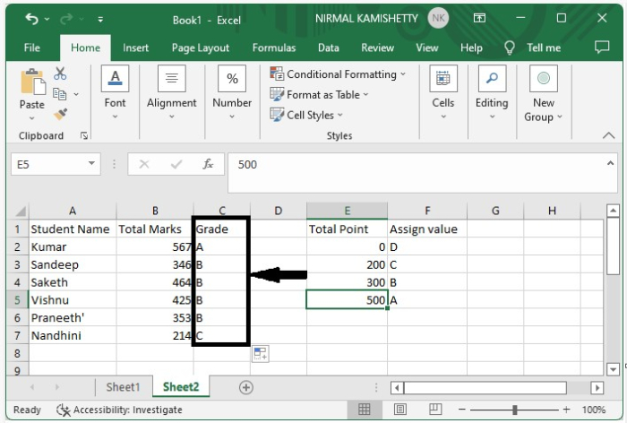
Step 2

We got the first result successfully, and we can get all the other results just by dragging from the first result until all the results are successfully printed, and our final result will be similar to the below image.

Conclusion

In this tutorial, we used a simple example to demonstrate how we can apply a value based on a number range in Excel to highlight a particular set of data.