H2O - Quick Guide

H2O - Introduction

Have you ever been asked to develop a Machine Learning model on a huge database? Typically, the customer will provide you the database and ask you to make certain predictions such as who will be the potential buyers; if there can be an early detection of fraudulent cases, etc. To answer these questions, your task would be to develop a Machine Learning algorithm that would provide an answer to the customer’s query. Developing a Machine Learning algorithm from scratch is not an easy task and why should you do this when there are several ready-to-use Machine Learning libraries available in the market.

These days, you would rather use these libraries, apply a well-tested algorithm from these libraries and look at its performance. If the performance were not within acceptable limits, you would try to either fine-tune the current algorithm or try an altogether different one.

Likewise, you may try multiple algorithms on the same dataset and then pick up the best one that satisfactorily meets the customer’s requirements. This is where H2O comes to your rescue. It is an open source Machine Learning framework with full-tested implementations of several widely-accepted ML algorithms. You just have to pick up the algorithm from its huge repository and apply it to your dataset. It contains the most widely used statistical and ML algorithms.

To mention a few here it includes gradient boosted machines (GBM), generalized linear model (GLM), deep learning and many more. Not only that it also supports AutoML functionality that will rank the performance of different algorithms on your dataset, thus reducing your efforts of finding the best performing model. H2O is used worldwide by more than 18000 organizations and interfaces well with R and Python for your ease of development. It is an in-memory platform that provides superb performance.

In this tutorial, you will first learn to install the H2O on your machine with both Python and R options. We will understand how to use this in the command line so that you understand its working line-wise. If you are a Python lover, you may use Jupyter or any other IDE of your choice for developing H2O applications. If you prefer R, you may use RStudio for development.

In this tutorial, we will consider an example to understand how to go about working with H2O. We will also learn how to change the algorithm in your program code and compare its performance with the earlier one. The H2O also provides a web-based tool to test the different algorithms on your dataset. This is called Flow.

The tutorial will introduce you to the use of Flow. Alongside, we will discuss the use of AutoML that will identify the best performing algorithm on your dataset. Are you not excited to learn H2O? Keep reading!

H2O - Installation

H2O can be configured and used with five different options as listed below −

Install in Python
Install in R
Web-based Flow GUI
Hadoop
Anaconda Cloud

In our subsequent sections, you will see the instructions for installation of H2O based on the options available. You are likely to use one of the options.

Install in Python

To run H2O with Python, the installation requires several dependencies. So let us start installing the minimum set of dependencies to run H2O.

Installing Dependencies

To install a dependency, execute the following pip command −

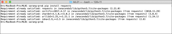
$ pip install requests

Open your console window and type the above command to install the requests package. The following screenshot shows the execution of the above command on our Mac machine −

After installing requests, you need to install three more packages as shown below −

$ pip install tabulate
$ pip install "colorama >= 0.3.8"
$ pip install future

The most updated list of dependencies is available on H2O GitHub page. At the time of this writing, the following dependencies are listed on the page.

python 2. H2O — Installation
pip >= 9.0.1
setuptools
colorama >= 0.3.7
future >= 0.15.2

Removing Older Versions

After installing the above dependencies, you need to remove any existing H2O installation. To do so, run the following command −

$ pip uninstall h2o

Installing the Latest Version

Now, let us install the latest version of H2O using the following command −

$ pip install -f http://h2o-release.s3.amazonaws.com/h2o/latest_stable_Py.html h2o

After successful installation, you should see the following message display on the screen −

Installing collected packages: h2o
Successfully installed h2o-3.26.0.1

Testing the Installation

To test the installation, we will run one of the sample applications provided in the H2O installation. First start the Python prompt by typing the following command −

$ Python3

Once the Python interpreter starts, type the following Python statement on the Python command prompt −

>>>import h2o

The above command imports the H2O package in your program. Next, initialize the H2O system using the following command −

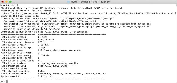
>>>h2o.init()

Your screen would show the cluster information and should look the following at this stage −

Now, you are ready to run the sample code. Type the following command on the Python prompt and execute it.

>>>h2o.demo("glm")

The demo consists of a Python notebook with a series of commands. After executing each command, its output is shown immediately on the screen and you will be asked to hit the key to continue with the next step. The partial screenshot on executing the last statement in the notebook is shown here −

At this stage your Python installation is complete and you are ready for your own experimentation.

Install in R

Installing H2O for R development is very much similar to installing it for Python, except that you would be using R prompt for the installation.

Starting R Console

Start R console by clicking on the R application icon on your machine. The console screen would appear as shown in the following screenshot −

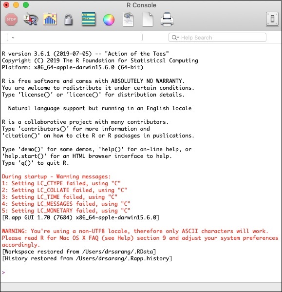
Your H2O installation would be done on the above R prompt. If you prefer using RStudio, type the commands in the R console subwindow.

Removing Older Versions

To begin with, remove older versions using the following command on the R prompt −

> if ("package:h2o" %in% search()) { detach("package:h2o", unload=TRUE) }
> if ("h2o" %in% rownames(installed.packages())) { remove.packages("h2o") }

Downloading Dependencies

Download the dependencies for H2O using the following code −

> pkgs <- c("RCurl","jsonlite")
for (pkg in pkgs) {
   if (! (pkg %in% rownames(installed.packages()))) { install.packages(pkg) }
}

Installing H2O

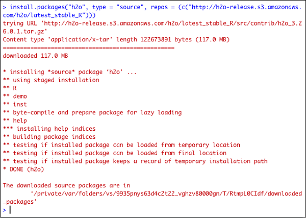
Install H2O by typing the following command on the R prompt −

> install.packages("h2o", type = "source", repos = (c("http://h2o-release.s3.amazonaws.com/h2o/latest_stable_R")))

The following screenshot shows the expected output −

There is another way of installing H2O in R.

Install in R from CRAN

To install R from CRAN, use the following command on R prompt −

> install.packages("h2o")

You will be asked to select the mirror −

--- Please select a CRAN mirror for use in this session ---

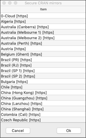
A dialog box displaying the list of mirror sites is shown on your screen. Select the nearest location or the mirror of your choice.

Testing Installation

On the R prompt, type and run the following code −

> library(h2o)
> localH2O = h2o.init()
> demo(h2o.kmeans)

The output generated will be as shown in the following screenshot −

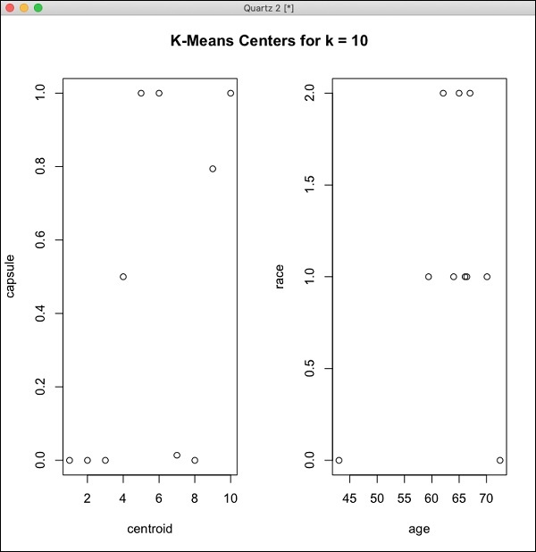
Your H2O installation in R is complete now.

Installing Web GUI Flow

To install GUI Flow download the installation file from the H20 site. Unzip the downloaded file in your preferred folder. Note the presence of h2o.jar file in the installation. Run this file in a command window using the following command −

$ java -jar h2o.jar

After a while, the following will appear in your console window.

07-24 16:06:37.304 192.168.1.18:54321 3294 main INFO: H2O started in 7725ms
07-24 16:06:37.304 192.168.1.18:54321 3294 main INFO:
07-24 16:06:37.305 192.168.1.18:54321 3294 main INFO: Open H2O Flow in your web browser: http://192.168.1.18:54321
07-24 16:06:37.305 192.168.1.18:54321 3294 main INFO:

To start the Flow, open the given URL http://localhost:54321 in your browser. The following screen will appear −

At this stage, your Flow installation is complete.

Install on Hadoop / Anaconda Cloud

Unless you are a seasoned developer, you would not think of using H2O on Big Data. It is sufficient to say here that H2O models run efficiently on huge databases of several terabytes. If your data is on your Hadoop installation or in the Cloud, follow the steps given on H2O site to install it for your respective database.

Now that you have successfully installed and tested H2O on your machine, you are ready for real development. First, we will see the development from a Command prompt. In our subsequent lessons, we will learn how to do model testing in H2O Flow.

Developing in Command Prompt

Let us now consider using H2O to classify plants of the well-known iris dataset that is freely available for developing Machine Learning applications.

Start the Python interpreter by typing the following command in your shell window −

$ Python3

This starts the Python interpreter. Import h2o platform using the following command −

>>> import h2o

We will use Random Forest algorithm for classification. This is provided in the H2ORandomForestEstimator package. We import this package using the import statement as follows −

>>> from h2o.estimators import H2ORandomForestEstimator

We initialize the H2o environment by calling its init method.

>>> h2o.init()

On successful initialization, you should see the following message on the console along with the cluster information.

Checking whether there is an H2O instance running at http://localhost:54321 . connected.

Now, we will import the iris data using the import_file method in H2O.

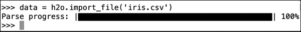
>>> data = h2o.import_file('iris.csv')

The progress will display as shown in the following screenshot −

After the file is loaded in the memory, you can verify this by displaying the first 10 rows of the loaded table. You use the head method to do so −

>>> data.head()

You will see the following output in tabular format.

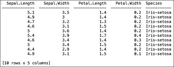
The table also displays the column names. We will use the first four columns as the features for our ML algorithm and the last column class as the predicted output. We specify this in the call to our ML algorithm by first creating the following two variables.

>>> features = ['sepal_length', 'sepal_width', 'petal_length', 'petal_width']
>>> output = 'class'

Next, we split the data into training and testing by calling the split_frame method.

>>> train, test = data.split_frame(ratios = [0.8])

The data is split in the 80:20 ratio. We use 80% data for training and 20% for testing.

Now, we load the built-in Random Forest model into the system.

>>> model = H2ORandomForestEstimator(ntrees = 50, max_depth = 20, nfolds = 10)

In the above call, we set the number of trees to 50, the maximum depth for the tree to 20 and number of folds for cross validation to 10. We now need to train the model. We do so by calling the train method as follows −

>>> model.train(x = features, y = output, training_frame = train)

The train method receives the features and the output that we created earlier as first two parameters. The training dataset is set to train, which is the 80% of our full dataset. During training, you will see the progress as shown here −

Now, as the model building process is over, it is time to test the model. We do this by calling the model_performance method on the trained model object.

>>> performance = model.model_performance(test_data=test)

In the above method call, we sent test data as our parameter.

It is time now to see the output, which is the performance of our model. You do this by simply printing the performance.

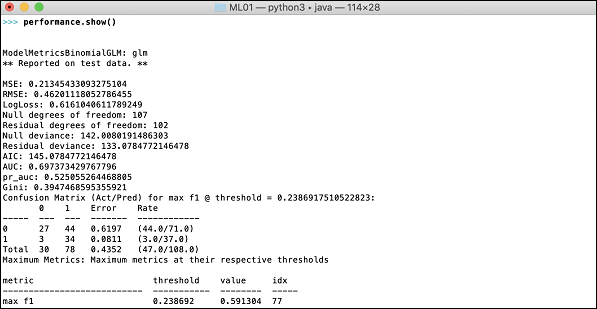
>>> print (performance)

This will give you the following output −

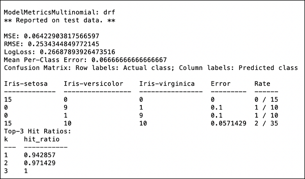
The output shows the Mean Square Error (MSE), Root Mean Square Error (RMSE), LogLoss and even the Confusion Matrix.

Running in Jupyter

We have seen the execution from the command and also understood the purpose of each line of code. You may run the entire code in a Jupyter environment, either line by line or the whole program at a time. The complete listing is given here −

import h2o
from h2o.estimators import H2ORandomForestEstimator
h2o.init()
data = h2o.import_file('iris.csv')
features = ['sepal_length', 'sepal_width', 'petal_length', 'petal_width']
output = 'class'
train, test = data.split_frame(ratios=[0.8])
model = H2ORandomForestEstimator(ntrees = 50, max_depth = 20, nfolds = 10)
model.train(x = features, y = output, training_frame = train)
performance = model.model_performance(test_data=test)
print (performance)

Run the code and observe the output. You can now appreciate how easy it is to apply and test a Random Forest algorithm on your dataset. The power of H20 goes far beyond this capability. What if you want to try another model on the same dataset to see if you can get better performance. This is explained in our subsequent section.

Applying a Different Algorithm

Now, we will learn how to apply a Gradient Boosting algorithm to our earlier dataset to see how it performs. In the above full listing, you will need to make only two minor changes as highlighted in the code below −

import h2o 
from h2o.estimators import H2OGradientBoostingEstimator
h2o.init()
data = h2o.import_file('iris.csv')
features = ['sepal_length', 'sepal_width', 'petal_length', 'petal_width']
output = 'class'
train, test = data.split_frame(ratios = [0.8]) 
model = H2OGradientBoostingEstimator
(ntrees = 50, max_depth = 20, nfolds = 10)
model.train(x = features, y = output, training_frame = train)
performance = model.model_performance(test_data = test)
print (performance)

Run the code and you will get the following output −

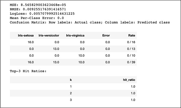
Just compare the results like MSE, RMSE, Confusion Matrix, etc. with the previous output and decide on which one to use for production deployment. As a matter of fact, you can apply several different algorithms to decide on the best one that meets your purpose.

H2O - Flow

In the last lesson, you learned to create H2O based ML models using command line interface. H2O Flow fulfils the same purpose, but with a web-based interface.

In the following lessons, I will show you how to start H2O Flow and to run a sample application.

Starting H2O Flow

The H2O installation that you downloaded earlier contains the h2o.jar file. To start H2O Flow, first run this jar from the command prompt −

$ java -jar h2o.jar

When the jar runs successfully, you will get the following message on the console −

Open H2O Flow in your web browser: http://192.168.1.10:54321

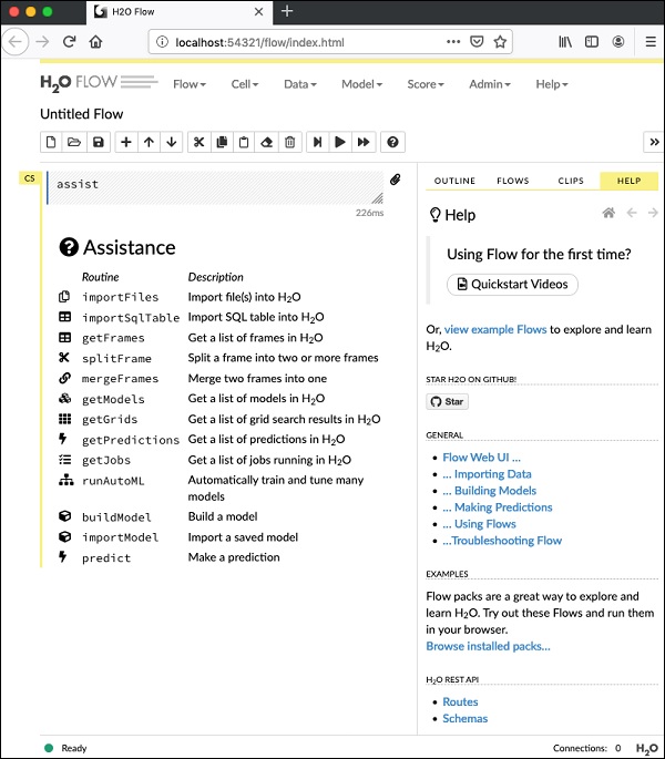
Now, open the browser of your choice and type the above URL. You would see the H2O web-based desktop as shown here −

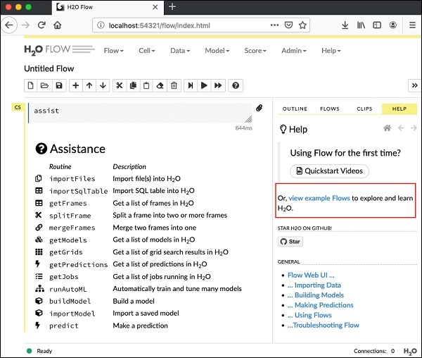
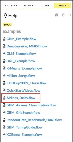
This is basically a notebook similar to Colab or Jupyter. I will show you how to load and run a sample application in this notebook while explaining the various features in Flow. Click on the view example Flows link on the above screen to see the list of provided examples.

I will describe the Airlines delay Flow example from the sample.

H2O - Running Sample Application

Click on the Airlines Delay Flow link in the list of samples as shown in the screenshot below −

After you confirm, the new notebook would be loaded.

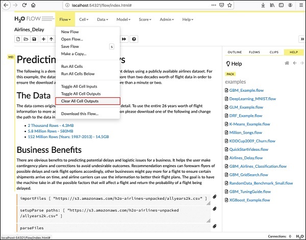
Clearing All Outputs

Before we explain the code statements in the notebook, let us clear all the outputs and then run the notebook gradually. To clear all outputs, select the following menu option −

Flow / Clear All Cell Contents

This is shown in the following screenshot −

Once all outputs are cleared, we will run each cell in the notebook individually and examine its output.

Running the First Cell

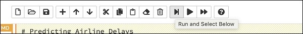
Click the first cell. A red flag appears on the left indicating that the cell is selected. This is as shown in the screenshot below −

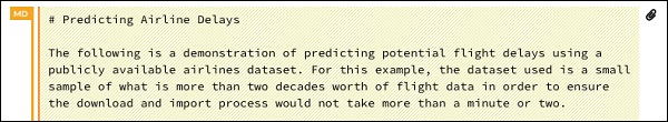
The contents of this cell are just the program comment written in MarkDown (MD) language. The content describes what the loaded application does. To run the cell, click the Run icon as shown in the screenshot below −

You will not see any output underneath the cell as there is no executable code in the current cell. The cursor now moves automatically to the next cell, which is ready to execute.

Importing Data

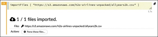
The next cell contains the following Python statement −

importFiles ["https://s3.amazonaws.com/h2o-airlines-unpacked/allyears2k.csv"]

The statement imports the allyears2k.csv file from Amazon AWS into the system. When you run the cell, it imports the file and gives you the following output.

Setting Up Data Parser

Now, we need to parse the data and make it suitable for our ML algorithm. This is done using the following command −

setupParse paths: [ "https://s3.amazonaws.com/h2o-airlines-unpacked/allyears2k.csv" ]

Upon execution of the above statement, a setup configuration dialog appears. The dialog allows you several settings for parsing the file. This is as shown in the screenshot below −

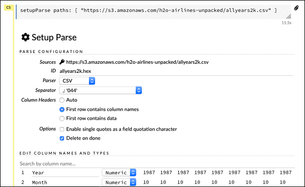
In this dialog, you can select the desired parser from the given drop-down list and set other parameters such as the field separator, etc.

Parsing Data

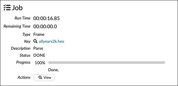
The next statement, which actually parses the datafile using the above configuration, is a long one and is as shown here −

parseFiles
paths: ["https://s3.amazonaws.com/h2o-airlines-unpacked/allyears2k.csv"]
destination_frame: "allyears2k.hex"
parse_type: "CSV"
separator: 44
number_columns: 31
single_quotes: false
column_names: ["Year","Month","DayofMonth","DayOfWeek","DepTime","CRSDepTime",
   "ArrTime","CRSArrTime","UniqueCarrier","FlightNum","TailNum",
   "ActualElapsedTime","CRSElapsedTime","AirTime","ArrDelay","DepDelay",
   "Origin","Dest","Distance","TaxiIn","TaxiOut","Cancelled","CancellationCode",
   "Diverted","CarrierDelay","WeatherDelay","NASDelay","SecurityDelay",
   "LateAircraftDelay","IsArrDelayed","IsDepDelayed"]
column_types: ["Enum","Enum","Enum","Enum","Numeric","Numeric","Numeric"
   ,"Numeric","Enum","Enum","Enum","Numeric","Numeric","Numeric","Numeric",
   "Numeric","Enum","Enum","Numeric","Numeric","Numeric","Enum","Enum",
   "Numeric","Numeric","Numeric","Numeric","Numeric","Numeric","Enum","Enum"]
delete_on_done: true
check_header: 1
chunk_size: 4194304

Observe that the parameters you have set up in the configuration box are listed in the above code. Now, run this cell. After a while, the parsing completes and you will see the following output −

Examining Dataframe

After the processing, it generates a dataframe, which can be examined using the following statement −

getFrameSummary "allyears2k.hex"

Upon execution of the above statement, you will see the following output −

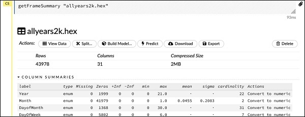
Now, your data is ready to be fed into a Machine Learning algorithm.

The next statement is a program comment that says we will be using the regression model and specifies the preset regularization and the lambda values.

Building the Model

Next, comes the most important statement and that is building the model itself. This is specified in the following statement −

buildModel 'glm', {
   "model_id":"glm_model","training_frame":"allyears2k.hex",
   "ignored_columns":[
      "DayofMonth","DepTime","CRSDepTime","ArrTime","CRSArrTime","TailNum",
      "ActualElapsedTime","CRSElapsedTime","AirTime","ArrDelay","DepDelay",
      "TaxiIn","TaxiOut","Cancelled","CancellationCode","Diverted","CarrierDelay",
      "WeatherDelay","NASDelay","SecurityDelay","LateAircraftDelay","IsArrDelayed"],
   "ignore_const_cols":true,"response_column":"IsDepDelayed","family":"binomial",
   "solver":"IRLSM","alpha":[0.5],"lambda":[0.00001],"lambda_search":false,
   "standardize":true,"non_negative":false,"score_each_iteration":false,
   "max_iterations":-1,"link":"family_default","intercept":true,
   "objective_epsilon":0.00001,"beta_epsilon":0.0001,"gradient_epsilon":0.0001,
   "prior":-1,"max_active_predictors":-1
}

We use glm, which is a Generalized Linear Model suite with family type set to binomial. You can see these highlighted in the above statement. In our case, the expected output is binary and that is why we use the binomial type. You may examine the other parameters by yourself; for example, look at alpha and lambda that we had specified earlier. Refer to the GLM model documentation for the explanation of all the parameters.

Now, run this statement. Upon execution, the following output will be generated −

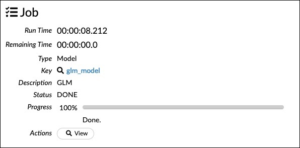
Certainly, the execution time would be different on your machine. Now, comes the most interesting part of this sample code.

Examining Output

We simply output the model that we have built using the following statement −

getModel "glm_model"

Note the glm_model is the model ID that we specified as model_id parameter while building the model in the previous statement. This gives us a huge output detailing the results with several varying parameters. A partial output of the report is shown in the screenshot below −

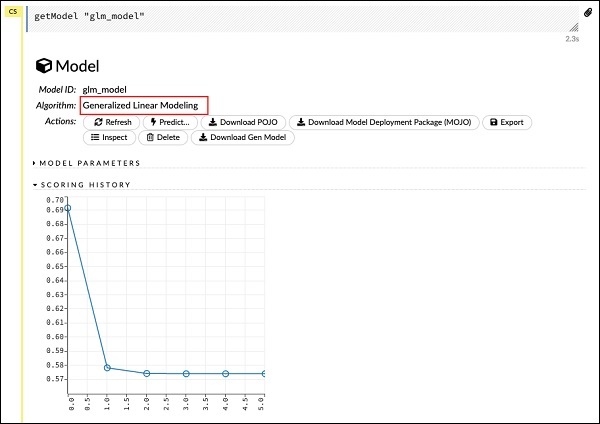
As you can see in the output, it says that this is the result of running the Generalized Linear Modeling algorithm on your dataset.

Right above the SCORING HISTORY, you see the MODEL PARAMETERS tag, expand it and you will see the list of all parameters that are used while building the model. This is shown in the screenshot below.

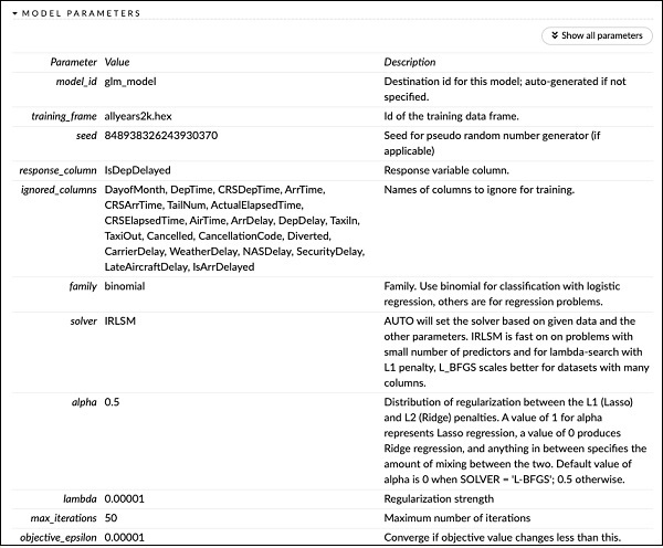
Likewise, each tag provides a detailed output of a specific type. Expand the various tags yourself to study the outputs of different kinds.

Building Another Model

Next, we will build a Deep Learning model on our dataframe. The next statement in the sample code is just a program comment. The following statement is actually a model building command. It is as shown here −

buildModel 'deeplearning', {
   "model_id":"deeplearning_model","training_frame":"allyear
   s2k.hex","ignored_columns":[
      "DepTime","CRSDepTime","ArrTime","CRSArrTime","FlightNum","TailNum",
      "ActualElapsedTime","CRSElapsedTime","AirTime","ArrDelay","DepDelay",
      "TaxiIn","TaxiOut","Cancelled","CancellationCode","Diverted",
      "CarrierDelay","WeatherDelay","NASDelay","SecurityDelay",
      "LateAircraftDelay","IsArrDelayed"],
   "ignore_const_cols":true,"res   ponse_column":"IsDepDelayed",
   "activation":"Rectifier","hidden":[200,200],"epochs":"100",
   "variable_importances":false,"balance_classes":false,
   "checkpoint":"","use_all_factor_levels":true,
   "train_samples_per_iteration":-2,"adaptive_rate":true,
   "input_dropout_ratio":0,"l1":0,"l2":0,"loss":"Automatic","score_interval":5,
   "score_training_samples":10000,"score_duty_cycle":0.1,"autoencoder":false,
   "overwrite_with_best_model":true,"target_ratio_comm_to_comp":0.02,
   "seed":6765686131094811000,"rho":0.99,"epsilon":1e-8,"max_w2":"Infinity",
   "initial_weight_distribution":"UniformAdaptive","classification_stop":0,
   "diagnostics":true,"fast_mode":true,"force_load_balance":true,
   "single_node_mode":false,"shuffle_training_data":false,"missing_values_handling":
   "MeanImputation","quiet_mode":false,"sparse":false,"col_major":false,
   "average_activation":0,"sparsity_beta":0,"max_categorical_features":2147483647,
   "reproducible":false,"export_weights_and_biases":false
}

As you can see in the above code, we specify deeplearning for building the model with several parameters set to the appropriate values as specified in the documentation of deeplearning model. When you run this statement, it will take longer time than the GLM model building. You will see the following output when the model building completes, albeit with different timings.

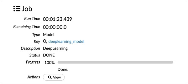
Examining Deep Learning Model Output

This generates the kind of output, which can be examined using the following statement as in the earlier case.

getModel "deeplearning_model"

We will consider the ROC curve output as shown below for quick reference.

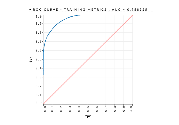
Like in the earlier case, expand the various tabs and study the different outputs.

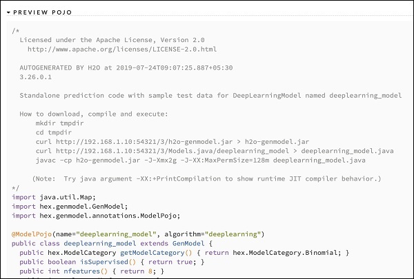
Saving the Model

After you have studied the output of different models, you decide to use one of those in your production environment. H20 allows you to save this model as a POJO (Plain Old Java Object).

Expand the last tag PREVIEW POJO in the output and you will see the Java code for your fine-tuned model. Use this in your production environment.

Next, we will learn about a very exciting feature of H2O. We will learn how to use AutoML to test and rank various algorithms based on their performance.

H2O - AutoML

To use AutoML, start a new Jupyter notebook and follow the steps shown below.

Importing AutoML

First import H2O and AutoML package into the project using the following two statements −

import h2o
from h2o.automl import H2OAutoML

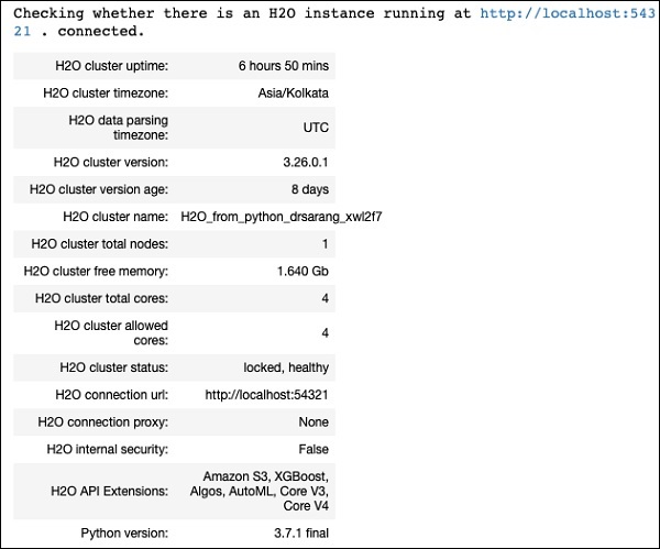
Initialize H2O

Initialize h2o using the following statement −

h2o.init()

You should see the cluster information on the screen as shown in the screenshot below −

Loading Data

We will use the same iris.csv dataset that you used earlier in this tutorial. Load the data using the following statement −

data = h2o.import_file('iris.csv')

Preparing Dataset

We need to decide on the features and the prediction columns. We use the same features and the predication column as in our earlier case. Set the features and the output column using the following two statements −

features = ['sepal_length', 'sepal_width', 'petal_length', 'petal_width']
output = 'class'

Split the data in 80:20 ratio for training and testing −

train, test = data.split_frame(ratios=[0.8])

Applying AutoML

Now, we are all set for applying AutoML on our dataset. The AutoML will run for a fixed amount of time set by us and give us the optimized model. We set up the AutoML using the following statement −

aml = H2OAutoML(max_models = 30, max_runtime_secs=300, seed = 1)

The first parameter specifies the number of models that we want to evaluate and compare.

The second parameter specifies the time for which the algorithm runs.

We now call the train method on the AutoML object as shown here −

aml.train(x = features, y = output, training_frame = train)

We specify the x as the features array that we created earlier, the y as the output variable to indicate the predicted value and the dataframe as train dataset.

Run the code, you will have to wait for 5 minutes (we set the max_runtime_secs to 300) until you get the following output −

Printing the Leaderboard

When the AutoML processing completes, it creates a leaderboard ranking all the 30 algorithms that it has evaluated. To see the first 10 records of the leaderboard, use the following code −

lb = aml.leaderboard
lb.head()

Upon execution, the above code will generate the following output −

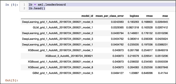
Clearly, the DeepLearning algorithm has got the maximum score.

Predicting on Test Data

Now, you have the models ranked, you can see the performance of the top-rated model on your test data. To do so, run the following code statement −

preds = aml.predict(test)

The processing continues for a while and you will see the following output when it completes.

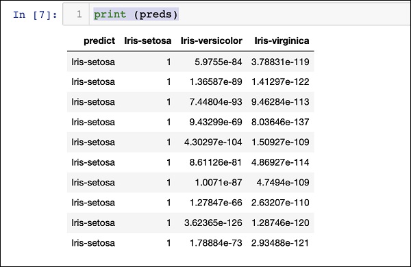
Printing Result

Print the predicted result using the following statement −

print (preds)

Upon execution of the above statement, you will see the following result −

Printing the Ranking for All

If you want to see the ranks of all the tested algorithms, run the following code statement −

lb.head(rows = lb.nrows)

Upon execution of the above statement, the following output will be generated (partially shown) −

Conclusion

H2O provides an easy-to-use open source platform for applying different ML algorithms on a given dataset. It provides several statistical and ML algorithms including deep learning. During testing, you can fine tune the parameters to these algorithms. You can do so using command-line or the provided web-based interface called Flow. H2O also supports AutoML that provides the ranking amongst the several algorithms based on their performance. H2O also performs well on Big Data. This is definitely a boon for Data Scientist to apply the different Machine Learning models on their dataset and pick up the best one to meet their needs.