Deep Learning with Keras - Quick Guide

---

---

Deep Learning with Keras - Introduction

Deep Learning has become a buzzword in recent days in the field of Artificial Intelligence (AI). For many years, we used Machine Learning (ML) for imparting intelligence to machines. In recent days, deep learning has become more popular due to its supremacy in predictions as compared to traditional ML techniques.

Deep Learning essentially means training an Artificial Neural Network (ANN) with a huge amount of data. In deep learning, the network learns by itself and thus requires humongous data for learning. While traditional machine learning is essentially a set of algorithms that parse data and learn from it. They then used this learning for making intelligent decisions.

Now, coming to Keras, it is a high-level neural networks API that runs on top of TensorFlow - an end-to-end open source machine learning platform. Using Keras, you easily define complex ANN architectures to experiment on your big data. Keras also supports GPU, which becomes essential for processing huge amount of data and developing machine learning models.

In this tutorial, you will learn the use of Keras in building deep neural networks. We shall look at the practical examples for teaching. The problem at hand is recognizing handwritten digits using a neural network that is trained with deep learning.

Just to get you more excited in deep learning, below is a screenshot of Google trends on deep learning here −

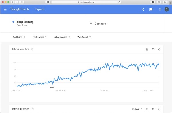
As you can see from the diagram, the interest in deep learning is steadily growing over the last several years. There are many areas such as computer vision, natural language processing, speech recognition, bioinformatics, drug design, and so on, where the deep learning has been successfully applied. This tutorial will get you quickly started on deep learning.

So keep reading!

Deep Learning with Keras - Deep Learning

As said in the introduction, deep learning is a process of training an artificial neural network with a huge amount of data. Once trained, the network will be able to give us the predictions on unseen data. Before I go further in explaining what deep learning is, let us quickly go through some terms used in training a neural network.

Neural Networks

The idea of artificial neural network was derived from neural networks in our brain. A typical neural network consists of three layers — input, output and hidden layer as shown in the picture below.

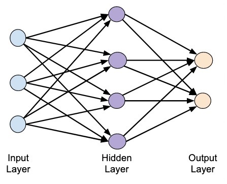
This is also called a shallow neural network, as it contains only one hidden layer. You add more hidden layers in the above architecture to create a more complex architecture.

Deep Networks

The following diagram shows a deep network consisting of four hidden layers, an input layer and an output layer.

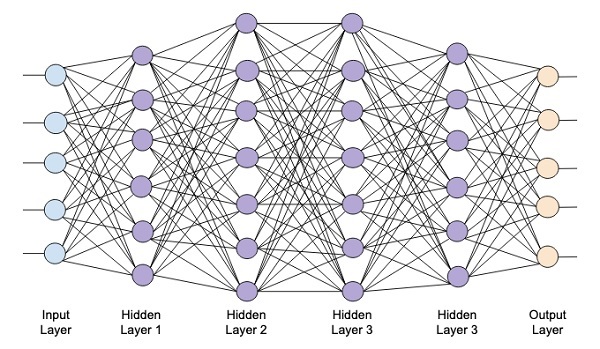
As the number of hidden layers are added to the network, its training becomes more complex in terms of required resources and the time it takes to fully train the network.

Network Training

After you define the network architecture, you train it for doing certain kinds of predictions. Training a network is a process of finding the proper weights for each link in the network. During training, the data flows from Input to Output layers through various hidden layers. As the data always moves in one direction from input to output, we call this network as Feed-forward Network and we call the data propagation as Forward Propagation.

Activation Function

At each layer, we calculate the weighted sum of inputs and feed it to an Activation function. The activation function brings nonlinearity to the network. It is simply some mathematical function that discretizes the output. Some of the most commonly used activations functions are sigmoid, hyperbolic, tangent (tanh), ReLU and Softmax.

Backpropagation

Backpropagation is an algorithm for supervised learning. In Backpropagation, the errors propagate backwards from the output to the input layer. Given an error function, we calculate the gradient of the error function with respect to the weights assigned at each connection. The calculation of the gradient proceeds backwards through the network. The gradient of the final layer of weights is calculated first and the gradient of the first layer of weights is calculated last.

At each layer, the partial computations of the gradient are reused in the computation of the gradient for the previous layer. This is called Gradient Descent.

In this project-based tutorial you will define a feed-forward deep neural network and train it with backpropagation and gradient descent techniques. Luckily, Keras provides us all high level APIs for defining network architecture and training it using gradient descent. Next, you will learn how to do this in Keras.

Handwritten Digit Recognition System

In this mini project, you will apply the techniques described earlier. You will create a deep learning neural network that will be trained for recognizing handwritten digits. In any machine learning project, the first challenge is collecting the data. Especially, for deep learning networks, you need humongous data. Fortunately, for the problem that we are trying to solve, somebody has already created a dataset for training. This is called mnist, which is available as a part of Keras libraries. The dataset consists of several 28x28 pixel images of handwritten digits. You will train your model on the major portion of this dataset and the rest of the data would be used for validating your trained model.

Project Description

The mnist dataset consists of 70000 images of handwritten digits. A few sample images are reproduced here for your reference

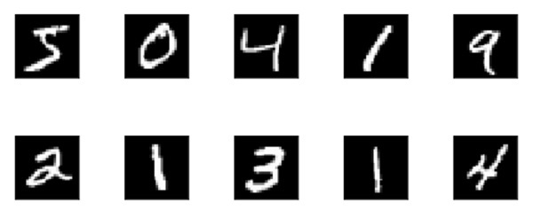
Each image is of size 28 x 28 pixels making it a total of 768 pixels of various gray scale levels. Most of the pixels tend towards black shade while only few of them are towards white. We will put the distribution of these pixels in an array or a vector. For example, the distribution of pixels for a typical image of digits 4 and 5 is shown in the figure below.

Each image is of size 28 x 28 pixels making it a total of 768 pixels of various gray scale levels. Most of the pixels tend towards black shade while only few of them are towards white. We will put the distribution of these pixels in an array or a vector. For example, the distribution of pixels for a typical image of digits 4 and 5 is shown in the figure below.

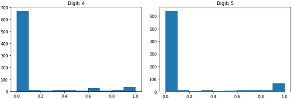
Clearly, you can see that the distribution of the pixels (especially those tending towards white tone) differ, this distinguishes the digits they represent. We will feed this distribution of 784 pixels to our network as its input. The output of the network will consist of 10 categories representing a digit between 0 and 9.

Our network will consist of 4 layers — one input layer, one output layer and two hidden layers. Each hidden layer will contain 512 nodes. Each layer is fully connected to the next layer. When we train the network, we will be computing the weights for each connection. We train the network by applying backpropagation and gradient descent that we discussed earlier.

Deep Learning with Keras - Setting up Project

With this background, let us now start creating the project.

Setting Up Project

We will use Jupyter through Anaconda navigator for our project. As our project uses TensorFlow and Keras, you will need to install those in Anaconda setup. To install Tensorflow, run the following command in your console window:

>conda install -c anaconda tensorflow

To install Keras, use the following command −

>conda install -c anaconda keras

You are now ready to start Jupyter.

Starting Jupyter

When you start the Anaconda navigator, you would see the following opening screen.

Click ‘Jupyter’ to start it. The screen will show up the existing projects, if any, on your drive.

Starting a New Project

Start a new Python 3 project in Anaconda by selecting the following menu option −

File | New Notebook | Python 3

The screenshot of the menu selection is shown for your quick reference −

A new blank project will show up on your screen as shown below −

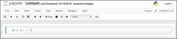
Change the project name to DeepLearningDigitRecognition by clicking and editing on the default name “UntitledXX”.

Deep Learning with Keras - Importing Libraries

We first import the various libraries required by the code in our project.

Array Handling and Plotting

As typical, we use numpy for array handling and matplotlib for plotting. These libraries are imported in our project using the following import statements

import numpy as np
import matplotlib
import matplotlib.pyplot as plot

Suppressing Warnings

As both Tensorflow and Keras keep on revising, if you do not sync their appropriate versions in the project, at runtime you would see plenty of warning errors. As they distract your attention from learning, we shall be suppressing all the warnings in this project. This is done with the following lines of code −

# silent all warnings
import os
os.environ['TF_CPP_MIN_LOG_LEVEL']='3'
import warnings
warnings.filterwarnings('ignore')
from tensorflow.python.util import deprecation
deprecation._PRINT_DEPRECATION_WARNINGS = False

Keras

We use Keras libraries to import dataset. We will use the mnist dataset for handwritten digits. We import the required package using the following statement

from keras.datasets import mnist

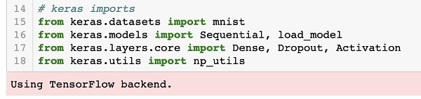
We will be defining our deep learning neural network using Keras packages. We import the Sequential, Dense, Dropout and Activation packages for defining the network architecture. We use load_model package for saving and retrieving our model. We also use np_utils for a few utilities that we need in our project. These imports are done with the following program statements −

from keras.models import Sequential, load_model
from keras.layers.core import Dense, Dropout, Activation
from keras.utils import np_utils

When you run this code, you will see a message on the console that says that Keras uses TensorFlow at the backend. The screenshot at this stage is shown here −

Now, as we have all the imports required by our project, we will proceed to define the architecture for our Deep Learning network.

Creating Deep Learning Model

Our neural network model will consist of a linear stack of layers. To define such a model, we call the Sequential function −

model = Sequential()

Input Layer

We define the input layer, which is the first layer in our network using the following program statement −

model.add(Dense(512, input_shape=(784,)))

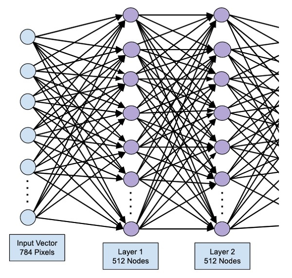
This creates a layer with 512 nodes (neurons) with 784 input nodes. This is depicted in the figure below −

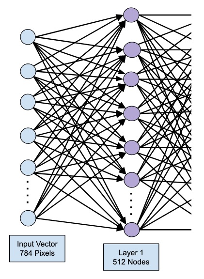
Note that all the input nodes are fully connected to the Layer 1, that is each input node is connected to all 512 nodes of Layer 1.

Next, we need to add the activation function for the output of Layer 1. We will use ReLU as our activation. The activation function is added using the following program statement −

model.add(Activation('relu'))

Next, we add Dropout of 20% using the statement below. Dropout is a technique used to prevent model from overfitting.

model.add(Dropout(0.2))

At this point, our input layer is fully defined. Next, we will add a hidden layer.

Hidden Layer

Our hidden layer will consist of 512 nodes. The input to the hidden layer comes from our previously defined input layer. All the nodes are fully connected as in the earlier case. The output of the hidden layer will go to the next layer in the network, which is going to be our final and output layer. We will use the same ReLU activation as for the previous layer and a dropout of 20%. The code for adding this layer is given here −

model.add(Dense(512))
model.add(Activation('relu'))
model.add(Dropout(0.2))

The network at this stage can be visualized as follows −

Next, we will add the final layer to our network, which is the output layer. Note that you may add any number of hidden layers using the code similar to the one which you have used here. Adding more layers would make the network complex for training; however, giving a definite advantage of better results in many cases though not all.

Output Layer

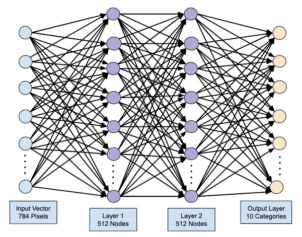
The output layer consists of just 10 nodes as we want to classify the given images in 10 distinct digits. We add this layer, using the following statement −

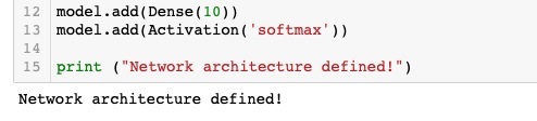
model.add(Dense(10))

As we want to classify the output in 10 distinct units, we use the softmax activation. In case of ReLU, the output is binary. We add the activation using the following statement −

model.add(Activation('softmax'))

At this point, our network can be visualized as shown in the below diagram −

At this point, our network model is fully defined in the software. Run the code cell and if there are no errors, you will get a confirmation message on the screen as shown in the screenshot below −

Next, we need to compile the model.

Deep Learning with Keras - Compiling the Model

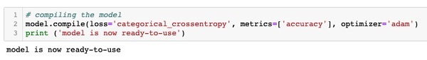
The compilation is performed using one single method call called compile.

model.compile(loss='categorical_crossentropy', metrics=['accuracy'], optimizer='adam')

The compile method requires several parameters. The loss parameter is specified to have type 'categorical_crossentropy'. The metrics parameter is set to 'accuracy' and finally we use the adam optimizer for training the network. The output at this stage is shown below −

Now, we are ready to feed in the data to our network.

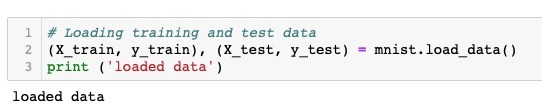
Loading Data

As said earlier, we will use the mnist dataset provided by Keras. When we load the data into our system, we will split it in the training and test data. The data is loaded by calling the load_data method as follows −

(X_train, y_train), (X_test, y_test) = mnist.load_data()

The output at this stage looks like the following −

Now, we shall learn the structure of the loaded dataset.

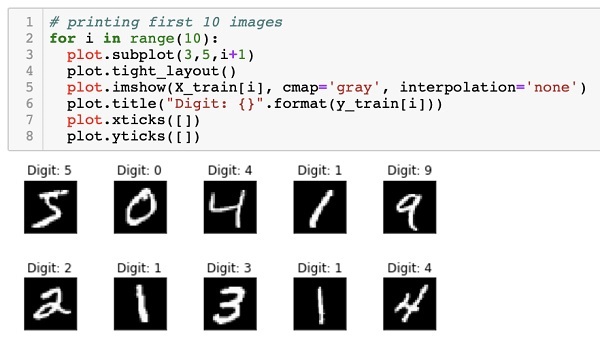
The data that is provided to us are the graphic images of size 28 x 28 pixels, each containing a single digit between 0 and 9. We will display the first ten images on the console. The code for doing so is given below −

# printing first 10 images
for i in range(10):

plot.subplot(3,5,i+1)
plot.tight_layout()
plot.imshow(X_train[i], cmap='gray', interpolation='none')
plot.title("Digit: {}".format(y_train[i]))
plot.xticks([])
plot.yticks([])

In an iterative loop of 10 counts, we create a subplot on each iteration and show an image from X_train vector in it. We title each image from the corresponding y_train vector. Note that the y_train vector contains the actual values for the corresponding image in X_train vector. We remove the x and y axes markings by calling the two methods xticks and yticks with null argument. When you run the code, you would see the following output −

Next, we will prepare data for feeding it into our network.

Deep Learning with Keras - Preparing Data

Before we feed the data to our network, it must be converted into the format required by the network. This is called preparing data for the network. It generally consists of converting a multi-dimensional input to a single-dimension vector and normalizing the data points.

Reshaping Input Vector

The images in our dataset consist of 28 x 28 pixels. This must be converted into a single dimensional vector of size 28 * 28 = 784 for feeding it into our network. We do so by calling the reshape method on the vector.

X_train = X_train.reshape(60000, 784)
X_test = X_test.reshape(10000, 784)

Now, our training vector will consist of 60000 data points, each consisting of a single dimension vector of size 784. Similarly, our test vector will consist of 10000 data points of a single-dimension vector of size 784.

Normalizing Data

The data that the input vector contains currently has a discrete value between 0 and 255 - the gray scale levels. Normalizing these pixel values between 0 and 1 helps in speeding up the training. As we are going to use stochastic gradient descent, normalizing data will also help in reducing the chance of getting stuck in local optima.

To normalize the data, we represent it as float type and divide it by 255 as shown in the following code snippet −

X_train = X_train.astype('float32')
X_test = X_test.astype('float32')
X_train /= 255
X_test /= 255

Let us now look at how the normalized data looks like.

Examining Normalized Data

To view the normalized data, we will call the histogram function as shown here −

plot.hist(X_train[0])
plot.title("Digit: {}".format(y_train[0]))

Here, we plot the histogram of the first element of the X_train vector. We also print the digit represented by this data point. The output of running the above code is shown here −

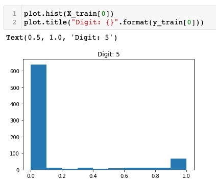
You will notice a thick density of points having value close to zero. These are the black dot points in the image, which obviously is the major portion of the image. The rest of the gray scale points, which are close to white color, represent the digit. You may check out the distribution of pixels for another digit. The code below prints the histogram of a digit at index of 2 in the training dataset.

plot.hist(X_train[2])
plot.title("Digit: {}".format(y_train[2])

The output of running the above code is shown below −

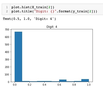
Comparing the above two figures, you will notice that the distribution of the white pixels in two images differ indicating a representation of a different digit - “5” and “4” in the above two pictures.

Next, we will examine the distribution of data in our full training dataset.

Examining Data Distribution

Before we train our machine learning model on our dataset, we should know the distribution of unique digits in our dataset. Our images represent 10 distinct digits ranging from 0 to 9. We would like to know the number of digits 0, 1, etc., in our dataset. We can get this information by using the unique method of Numpy.

Use the following command to print the number of unique values and the number of occurrences of each one

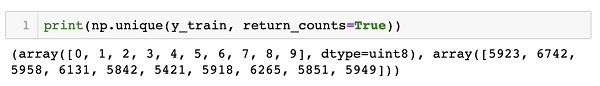
print(np.unique(y_train, return_counts=True))

When you run the above command, you will see the following output −

(array([0, 1, 2, 3, 4, 5, 6, 7, 8, 9], dtype=uint8), array([5923, 6742, 5958, 6131, 5842, 5421, 5918, 6265, 5851, 5949]))

It shows that there are 10 distinct values — 0 through 9. There are 5923 occurrences of digit 0, 6742 occurrences of digit 1, and so on. The screenshot of the output is shown here −

As a final step in data preparation, we need to encode our data.

Encoding Data

We have ten categories in our dataset. We will thus encode our output in these ten categories using one-hot encoding. We use to_categorial method of Numpy utilities to perform encoding. After the output data is encoded, each data point would be converted into a single dimensional vector of size 10. For example, digit 5 will now be represented as [0,0,0,0,0,1,0,0,0,0].

Encode the data using the following piece of code −

n_classes = 10
Y_train = np_utils.to_categorical(y_train, n_classes)

You may check out the result of encoding by printing the first 5 elements of the categorized Y_train vector.

Use the following code to print the first 5 vectors −

for i in range(5):
   print (Y_train[i])

You will see the following output −

[0. 0. 0. 0. 0. 1. 0. 0. 0. 0.]
[1. 0. 0. 0. 0. 0. 0. 0. 0. 0.]
[0. 0. 0. 0. 1. 0. 0. 0. 0. 0.]
[0. 1. 0. 0. 0. 0. 0. 0. 0. 0.]
[0. 0. 0. 0. 0. 0. 0. 0. 0. 1.]

The first element represents digit 5, the second represents digit 0, and so on.

Finally, you will have to categorize the test data too, which is done using the following statement −

Y_test = np_utils.to_categorical(y_test, n_classes)

At this stage, your data is fully prepared for feeding into the network.

Next, comes the most important part and that is training our network model.

Deep Learning with Keras - Training the Model

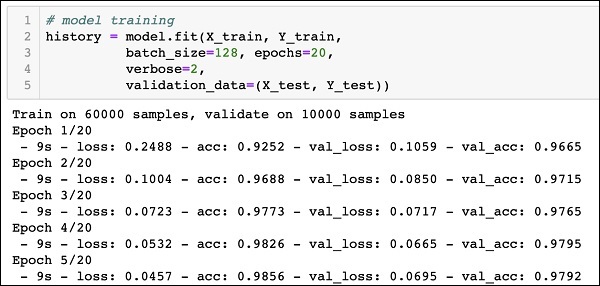
The model training is done in one single method call called fit that takes few parameters as seen in the code below −

history = model.fit(X_train, Y_train,
   batch_size=128, epochs=20,
   verbose=2,
   validation_data=(X_test, Y_test)))

The first two parameters to the fit method specify the features and the output of the training dataset.

The epochs is set to 20; we assume that the training will converge in max 20 epochs - the iterations. The trained model is validated on the test data as specified in the last parameter.

The partial output of running the above command is shown here −

Train on 60000 samples, validate on 10000 samples
Epoch 1/20
- 9s - loss: 0.2488 - acc: 0.9252 - val_loss: 0.1059 - val_acc: 0.9665
Epoch 2/20
- 9s - loss: 0.1004 - acc: 0.9688 - val_loss: 0.0850 - val_acc: 0.9715
Epoch 3/20
- 9s - loss: 0.0723 - acc: 0.9773 - val_loss: 0.0717 - val_acc: 0.9765
Epoch 4/20
- 9s - loss: 0.0532 - acc: 0.9826 - val_loss: 0.0665 - val_acc: 0.9795
Epoch 5/20
- 9s - loss: 0.0457 - acc: 0.9856 - val_loss: 0.0695 - val_acc: 0.9792

The screenshot of the output is given below for your quick reference −

Now, as the model is trained on our training data, we will evaluate its performance.

Evaluating Model Performance

To evaluate the model performance, we call evaluate method as follows −

loss_and_metrics = model.evaluate(X_test, Y_test, verbose=2)

To evaluate the model performance, we call evaluate method as follows −

loss_and_metrics = model.evaluate(X_test, Y_test, verbose=2)

We will print the loss and accuracy using the following two statements −

print("Test Loss", loss_and_metrics[0])
print("Test Accuracy", loss_and_metrics[1])

When you run the above statements, you would see the following output −

Test Loss 0.08041584826191042
Test Accuracy 0.9837

This shows a test accuracy of 98%, which should be acceptable to us. What it means to us that in 2% of the cases, the handwritten digits would not be classified correctly. We will also plot accuracy and loss metrics to see how the model performs on the test data.

Plotting Accuracy Metrics

We use the recorded history during our training to get a plot of accuracy metrics. The following code will plot the accuracy on each epoch. We pick up the training data accuracy (“acc”) and the validation data accuracy (“val_acc”) for plotting.

plot.subplot(2,1,1)
plot.plot(history.history['acc'])
plot.plot(history.history['val_acc'])
plot.title('model accuracy')
plot.ylabel('accuracy')
plot.xlabel('epoch')
plot.legend(['train', 'test'], loc='lower right')

The output plot is shown below −

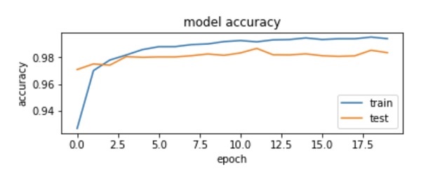
As you can see in the diagram, the accuracy increases rapidly in the first two epochs, indicating that the network is learning fast. Afterwards, the curve flattens indicating that not too many epochs are required to train the model further. Generally, if the training data accuracy (“acc”) keeps improving while the validation data accuracy (“val_acc”) gets worse, you are encountering overfitting. It indicates that the model is starting to memorize the data.

We will also plot the loss metrics to check our model’s performance.

Plotting Loss Metrics

Again, we plot the loss on both the training (“loss”) and test (“val_loss”) data. This is done using the following code −

plot.subplot(2,1,2)
plot.plot(history.history['loss'])
plot.plot(history.history['val_loss'])
plot.title('model loss')
plot.ylabel('loss')
plot.xlabel('epoch')
plot.legend(['train', 'test'], loc='upper right')

The output of this code is shown below −

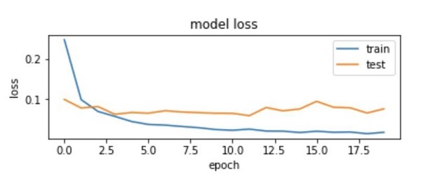
As you can see in the diagram, the loss on the training set decreases rapidly for the first two epochs. For the test set, the loss does not decrease at the same rate as the training set, but remains almost flat for multiple epochs. This means our model is generalizing well to unseen data.

Now, we will use our trained model to predict the digits in our test data.

Predicting on Test Data

To predict the digits in an unseen data is very easy. You simply need to call the predict_classes method of the model by passing it to a vector consisting of your unknown data points.

predictions = model.predict_classes(X_test)

The method call returns the predictions in a vector that can be tested for 0’s and 1’s against the actual values. This is done using the following two statements −

correct_predictions = np.nonzero(predictions == y_test)[0]
incorrect_predictions = np.nonzero(predictions != y_test)[0]

Finally, we will print the count of correct and incorrect predictions using the following two program statements −

print(len(correct_predictions)," classified correctly")
print(len(incorrect_predictions)," classified incorrectly")

When you run the code, you will get the following output −

9837 classified correctly
163 classified incorrectly

Now, as you have satisfactorily trained the model, we will save it for future use.

Deep Learning with Keras - Saving Model

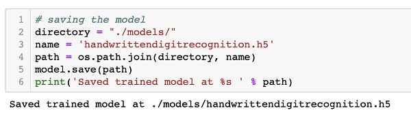
We will save the trained model in our local drive in the models folder in our current working directory. To save the model, run the following code −

directory = "./models/"
name = 'handwrittendigitrecognition.h5'
path = os.path.join(save_dir, name)
model.save(path)
print('Saved trained model at %s ' % path)

The output after running the code is shown below −

Now, as you have saved a trained model, you may use it later on for processing your unknown data.

Loading Model for Predictions

To predict the unseen data, you first need to load the trained model into the memory. This is done using the following command −

model = load_model ('./models/handwrittendigitrecognition.h5')

Note that we are simply loading the .h5 file into memory. This sets up the entire neural network in memory along with the weights assigned to each layer.

Now, to do your predictions on unseen data, load the data, let it be one or more items, into the memory. Preprocess the data to meet the input requirements of our model as what you did on your training and test data above. After preprocessing, feed it to your network. The model will output its prediction.

Deep Learning with Keras - Conclusion

Keras provides a high level API for creating deep neural network. In this tutorial, you learned to create a deep neural network that was trained for finding the digits in handwritten text. A multi-layer network was created for this purpose. Keras allows you to define an activation function of your choice at each layer. Using gradient descent, the network was trained on the training data. The accuracy of the trained network in predicting the unseen data was tested on the test data. You learned to plot the accuracy and error metrics. After the network is fully trained, you saved the network model for future use.