- Seaborn - Home
- Seaborn - Introduction
- Seaborn - Environment Setup
- Importing Datasets and Libraries
- Seaborn - Figure Aesthetic
- Seaborn- Color Palette
- Seaborn - Histogram
- Seaborn - Kernel Density Estimates
- Seaborn - Visualizing Pairwise Relationship
- Seaborn - Plotting Categorical Data
- Distribution of Observations
- Seaborn - Statistical Estimation
- Seaborn - Plotting Wide Form Data
- Seaborn - Multi Panel Categorical Plots
- Seaborn - Linear Relationships
- Seaborn - Facet Grid
- Seaborn - Pair Grid
- Seaborn Function Reference
- Seaborn - Function Reference
- Relational Plots
- Distribution Plots
- Categorial plots
- Regression plots
- Matrix Plots
- Multi plot grids
- Themeing
- Color Palettes
- Palette widgets
- Utility Functions
- Seaborn Useful Resources
- Seaborn - Quick Guide
- Seaborn - cheatsheet
- Seaborn - Useful Resources
- Seaborn - Discussion
Seaborn - ecdfplot() method
The Seaborn.edcfplot() method is used to plot empirical cumulative distribution functions.
The percentage or count of observations in a dataset that fall below each distinct value is represented by an empirical cumulative distribution function. It has the benefit that each observation is immediately displayed, as opposed to a histogram or density plot, therefore no binning or smoothing settings need to be changed. It also makes it easier to compare different distributions directly.
A drawback is that there may be a lack of clarity, instinctively in the link between the plot's appearance and the fundamental characteristics of the distribution, such as its central tendency, variance, and existence of any bimodality.
Syntax
Following is the syntax of the seaborn.ecdfplot() method −
seaborn.ecdfplot(data=None, *, x=None, y=None, hue=None, weights=None, stat='proportion', complementary=False, palette=None, hue_order=None, hue_norm=None, log_scale=None, legend=True, ax=None, **kwargs
Parameters
Some of the parameters of the above-mentioned method are as follows.
| S.No | Parameter and Description |
|---|---|
| 1 | x,y Variables that are represented on the x,y axis. |
| 2 | Hue This will produce elements with different colors. It is a grouping variable. |
| 3 | Complementary This parameter is used to draw the complementary of the cumulative distribution function. i.e; 1-CDF. |
| 4 | Sta This parameter takes values proportion and count. It is the distribution statistic to compute. |
| 5 | palette This parameter sets the color of the plot when hue mapping is considered too. |
| 6 | Hue_order The order of plotting the categorical variables in hue semantic. |
| 7 | Hue_norm Used to set normalization range in data units for hue semantic. A pair of data values are provided. |
| 8 | Weights If this parameter is passed, these numbers are used to weight the respective data points' contribution to the cumulative distribution. |
| 9 | Log_scale Sets axes scales to log and the values plotted are in log scale. |
| 10 | Legend Boolean value. If false, does not print out the legend of semantic variables. |
let us load the seaborn library and the dataset before moving on to the developing the plots.
Loading the seaborn library
To load or import the seaborn library the following line of code can be used.
Import seaborn as sns
Loading the dataset
in this article, we will make use of the Tips dataset inbuilt in the seaborn library. the following command is used to load the dataset.
tips=sns.load_dataset("tips")
The below mentioned command is used to view the first 5 rows in the dataset. This enables us to understand what variables can be used to plot a graph.
tips.head()
the below is the output for the above piece of code.
index,total_bill,tip,sex,smoker,day,time,size
0,16.99,1.01,Female,No,Sun,Dinner,2
1,10.34,1.66,Male,No,Sun,Dinner,3
2,21.01,3.5,Male,No,Sun,Dinner,3
3,23.68,3.31,Male,No,Sun,Dinner,2
4,24.59,3.61,Female,No,Sun,Dinner,4
Now that we have loaded the data, we will move on to plotting the data.
Example 1
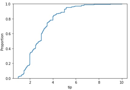
In this example, we will see how a empirical cumulative distribution function plot is plotted for a single variable in a dataset.
import seaborn as sns
import matplotlib.pyplot as plt
tips=sns.load_dataset("tips")
tips.head()
sns.ecdfplot(data=tips, x="tip")
plt.show()
Output
the output of the above code is seen below.
Example 2
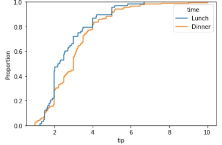
In this example, we will see the usage of the stat parameter. It can take values proportion and count. It is used to specify the distribution statistic to compute.
Passing proportion to the stat parameter. The code to do so is mentioned below.
import seaborn as sns
import matplotlib.pyplot as plt
tips=sns.load_dataset("tips")
tips.head()
sns.ecdfplot(data=tips, x="tip",hue="time",stat="proportion")
plt.show()
Output
The output of the following line of code is as follows
Passing count to the stat parameter. The code to so is mentioned below.
import seaborn as sns
import matplotlib.pyplot as plt
tips=sns.load_dataset("tips")
tips.head()
sns.ecdfplot(data=tips, x="tip",hue="time",stat="count")
plt.show()
Output
The output of the following line of code is as follows

Example 3
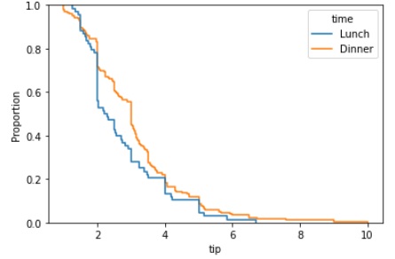
The complementary parameter of the seaborn.ecdfplot() method is used to draw the complementary of the cumulative distribution function and it is computed using 1-CDF. If it is True, then the complementary is printed. The same can be seen below.
import seaborn as sns
import matplotlib.pyplot as plt
tips=sns.load_dataset("tips")
tips.head()
sns.ecdfplot(data=tips, x="tip",hue="time",stat="proportion",complementary=True)
plt.show()
Output
the following output will be plotted for the above given code snippet.
Example 4
In this example, we will see how to not send any parameters but still be able to plot data on the screen.
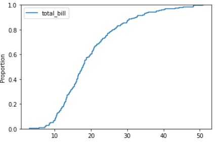
The dataset is handled as wide-form and a histogram is created for each numeric column if neither x nor y are assigned.
The below line of code can also be used in a scenario where there are multiple columns with the same name or beginning with the same name in a dataset.
import seaborn as sns
import matplotlib.pyplot as plt
tips=sns.load_dataset("tips")
tips.head()
sns.ecdfplot(data=tips.filter(like="total_", axis="columns"))
plt.show()
Output
the output for the code snippet is as follows.