- Electrical Machines - Home
- Basic Concepts
- Electromechanical Energy Conversion
- Energy Stored in Magnetic Field
- Singly-Excited and Doubly Excited Systems
- Rotating Electrical Machines
- Electrical Machines Types
- Faraday’s Laws of Electromagnetic Induction
- Concept of Induced EMF
- Fleming's Left Hand and Right Hand Rules
- Transformers
- Electrical Transformer
- Construction of Transformer
- EMF Equation of Transformer
- Turns Ratio and Voltage Transformation Ratio
- Ideal Transformer
- Practical Transformer
- Ideal and Practical Transformers
- Transformer on DC
- Losses in a Transformer
- Efficiency of Transformer
- 3-Phase Transformer
- Types of Transformers
- More on Transformers
- Transformer Working Principle
- Single-Phase Transformer Working Principle
- 3-Phase Transformer Principle
- 3-Phase Induction Motor Torque-Slip
- 3-Phase Induction Motor Torque-Speed
- 3-Phase Transformer Harmonics
- Double-Star Connection (3-6 Phase)
- Double-delta Connection (3-6 Phase)
- Transformer Ratios
- Voltage Regulation
- Delta-Star Connection (3-Phase)
- Star-Delta Connection (3-Phase)
- Autotransformer Conversion
- Back-to-back Test (Sumpner's Test)
- Transformer Voltage Drop
- Autotransformer Output
- Open and Short Circuit Test
- 3-Phase Autotransformer
- Star-Star Connection
- 6-Phase Diametrical Connections
- Circuit Test (Three-Winding)
- Potential Transformer
- Transformers Parallel Operation
- Open Delta (V-V) Connection
- Autotransformer
- Current Transformer
- No-Load Current Wave
- Transformer Inrush Current
- Transformer Vector Groups
- 3 to 12-Phase Transformers
- Scott-T Transformer Connection
- Transformer kVA Rating
- Three-Winding Transformer
- Delta-Delta Connection Transformer
- Transformer DC Supply Issue
- Equivalent Circuit Transformer
- Simplified Equivalent Circuit of Transformer
- Transformer No-Load Condition
- Transformer Load Condition
- OTI WTI Transformer
- CVT Transformer
- Isolation vs Regular Transformer
- Dry vs Oil-Filled
- DC Machines
- Construction of DC Machines
- Types of DC Machines
- Working Principle of DC Generator
- EMF Equation of DC Generator
- Derivation of EMF Equation DC Generator
- Types of DC Generators
- Working Principle of DC Motor
- Back EMF in DC Motor
- Types of DC Motors
- Losses in DC Machines
- Applications of DC Machines
- More on DC Machines
- DC Generator
- DC Generator Armature Reaction
- DC Generator Commutator Action
- Stepper vs DC Motors
- DC Shunt Generators Critical Resistance
- DC Machines Commutation
- DC Motor Characteristics
- Synchronous Generator Working Principle
- DC Generator Characteristics
- DC Generator Demagnetizing & Cross-Magnetizing
- DC Motor Voltage & Power Equations
- DC Generator Efficiency
- Electric Breaking of DC Motors
- DC Motor Efficiency
- Four Quadrant Operation of DC Motors
- Open Circuit Characteristics of DC Generators
- Voltage Build-Up in Self-Excited DC Generators
- Types of Armature Winding in DC Machines
- Torque in DC Motors
- Swinburne’s Test of DC Machine
- Speed Control of DC Shunt Motor
- Speed Control of DC Series Motor
- DC Motor of Speed Regulation
- Hopkinson's Test
- Permanent Magnet DC Motor
- Permanent Magnet Stepper Motor
- DC Servo Motor Theory
- DC Series vs Shunt Motor
- BLDC Motor vs PMSM Motor
- Induction Motors
- Introduction to Induction Motor
- Single-Phase Induction Motor
- 3-Phase Induction Motor
- Construction of 3-Phase Induction Motor
- 3-Phase Induction Motor on Load
- Characteristics of 3-Phase Induction Motor
- Speed Regulation and Speed Control
- Methods of Starting 3-Phase Induction Motors
- More on Induction Motors
- 3-Phase Induction Motor Working Principle
- 3-Phase Induction Motor Rotor Parameters
- Double Cage Induction Motor Equivalent Circuit
- Induction Motor Equivalent Circuit Models
- Slip Ring vs Squirrel Cage Induction Motors
- Single-Cage vs Double-Cage Induction Motor
- Induction Motor Equivalent Circuits
- Induction Motor Crawling & Cogging
- Induction Motor Blocked Rotor Test
- Induction Motor Circle Diagram
- 3-Phase Induction Motors Applications
- 3-Phase Induction Motors Torque Ratios
- Induction Motors Power Flow Diagram & Losses
- Determining Induction Motor Efficiency
- Induction Motor Speed Control by Pole-Amplitude Modulation
- Induction Motor Inverted or Rotor Fed
- High Torque Cage Motors
- Double-Cage Induction Motor Torque-Slip Characteristics
- 3-Phase Induction Motors Starting Torque
- 3-phase Induction Motor - Rotor Resistance Starter
- 3-phase Induction Motor Running Torque
- 3-Phase Induction Motor - Rotating Magnetic Field
- Isolated Induction Generator
- Capacitor-Start Induction Motor
- Capacitor-Start Capacitor-Run Induction Motor
- Winding EMFs in 3-Phase Induction Motors
- Split-Phase Induction Motor
- Shaded Pole Induction Motor
- Repulsion-Start Induction-Run Motor
- Repulsion Induction Motor
- PSC Induction Motor
- Single-Phase Induction Motor Performance Analysis
- Linear Induction Motor
- Single-Phase Induction Motor Testing
- 3-Phase Induction Motor Fault Types
- Synchronous Machines
- Introduction to 3-Phase Synchronous Machines
- Construction of Synchronous Machine
- Working of 3-Phase Alternator
- Armature Reaction in Synchronous Machines
- Output Power of 3-Phase Alternator
- Losses and Efficiency of an Alternator
- Losses and Efficiency of 3-Phase Alternator
- Working of 3-Phase Synchronous Motor
- Equivalent Circuit and Power Factor of Synchronous Motor
- Power Developed by Synchronous Motor
- More on Synchronous Machines
- AC Motor Types
- Induction Generator (Asynchronous Generator)
- Synchronous Speed Slip of 3-Phase Induction Motor
- Armature Reaction in Alternator at Leading Power Factor
- Armature Reaction in Alternator at Lagging Power Factor
- Stationary Armature vs Rotating Field Alternator Advantages
- Synchronous Impedance Method for Voltage Regulation
- Saturated & Unsaturated Synchronous Reactance
- Synchronous Reactance & Impedance
- Significance of Short Circuit Ratio in Alternator
- Hunting Effect Alternator
- Hydrogen Cooling in Synchronous Generators
- Excitation System of Synchronous Machine
- Equivalent Circuit Phasor Diagram of Synchronous Generator
- EMF Equation of Synchronous Generator
- Cooling Methods for Synchronous Generators
- Assumptions in Synchronous Impedance Method
- Armature Reaction at Unity Power Factor
- Voltage Regulation of Alternator
- Synchronous Generator with Infinite Bus Operation
- Zero Power Factor of Synchronous Generator
- Short Circuit Ratio Calculation of Synchronous Machines
- Speed-Frequency Relationship in Alternator
- Pitch Factor in Alternator
- Max Reactive Power in Synchronous Generators
- Power Flow Equations for Synchronous Generator
- Potier Triangle for Voltage Regulation in Alternators
- Parallel Operation of Alternators
- Load Sharing in Parallel Alternators
- Slip Test on Synchronous Machine
- Constant Flux Linkage Theorem
- Blondel's Two Reaction Theory
- Synchronous Machine Oscillations
- Ampere Turn Method for Voltage Regulation
- Salient Pole Synchronous Machine Theory
- Synchronization by Synchroscope
- Synchronization by Synchronizing Lamp Method
- Sudden Short Circuit in 3-Phase Alternator
- Short Circuit Transient in Synchronous Machines
- Power-Angle of Salient Pole Machines
- Prime-Mover Governor Characteristics
- Power Input of Synchronous Generator
- Power Output of Synchronous Generator
- Power Developed by Salient Pole Motor
- Phasor Diagrams of Cylindrical Rotor Moto
- Synchronous Motor Excitation Voltage Determination
- Hunting Synchronous Motor
- Self-Starting Synchronous Motor
- Unidirectional Torque Production in Synchronous Motor
- Effect of Load Change on Synchronous Motor
- Field Excitation Effect on Synchronous Motor
- Output Power of Synchronous Motor
- Input Power of Synchronous Motor
- V Curves & Inverted V Curves of Synchronous Motor
- Torque in Synchronous Motor
- Construction of 3-Phase Synchronous Motor
- Synchronous Motor
- Synchronous Condenser
- Power Flow in Synchronous Motor
- Types of Faults in Alternator
- Miscellaneous Topics
- Electrical Generator
- Determining Electric Motor Load
- Solid State Motor Starters
- Characteristics of Single-Phase Motor
- Types of AC Generators
- Three-Point Starter
- Four-Point Starter
- Ward Leonard Speed Control Method
- Pole Changing Method
- Stator Voltage Control Method
- DOL Starter
- Star-Delta Starter
- Hysteresis Motor
- 2-Phase & 3-Phase AC Servo Motors
- Repulsion Motor
- Reluctance Motor
- Stepper Motor
- PCB Motor
- Single-Stack Variable Reluctance Stepper Motor
- Schrage Motor
- Hybrid Schrage Motor
- Multi-Stack Variable Reluctance Stepper Motor
- Universal Motor
- Step Angle in Stepper Motor
- Stepper Motor Torque-Pulse Rate Characteristics
- Distribution Factor
- Electrical Machines Basic Terms
- Synchronizing Torque Coefficient
- Synchronizing Power Coefficient
- Metadyne
- Motor Soft Starter
- CVT vs PT
- Metering CT vs Protection CT
- Stator and Rotor in Electrical Machines
- Electric Motor Winding
- Electric Motor
- Useful Resources
- Quick Guide
- Resources
- Discussion
Power-Angle Characteristics of Salient Pole Synchronous Machine
Power-Angle Characteristics of Salient Pole Synchronous Machine
The resistance Ra of the armature can be neglected since it has negligible effect on the relationship between the power output of a synchronous machine and its torque angle δ. The phasor diagram at lagging power factor for a salient pole synchronous machine, neglecting Ra is shown in Figure-1. The power-angle characteristics of a salient-pole machine may be derived from the phasor diagram.

The complex power output per phase of the alternator is,
$$\mathrm{S_{1\phi} \:=\: V{I^{*}_{a}} \:\:\:\dotso\: (1)}$$
Taking excitation voltage (Ef) as the reference phasor, then,
$$\mathrm{V \:=\: V\:\angle -\delta \:=\: V\:\cos\delta \:-\: jV\:\sin\delta \:\:\:\dotso\: (2)}$$
$$\mathrm{I_{a} \:=\: I_{q} \:-\: jI_{d}}$$
$$\mathrm{\therefore\:{I^{*}_{a}} \:=\: I_{q} \:+\: jI_{d} \:\:\:\dotso\: (3)}$$
Hence, from Eqns. (1), (2) & (3), we get,
$$\mathrm{S_{1\phi} \:=\: (V\:\cos\delta \:-\: jV\:\sin\delta)(I_{q} \:+\: jI_{d}) \:\:\:\dotso\: (4)}$$
From the phasor diagram, we obtain,
$$\mathrm{CD \:=\: AM \:=\: I_{q}X_{q} \:=\: V\:\sin\delta}$$
$$\mathrm{\therefore\:I_{q} \:=\:\frac{V\:\sin\delta}{X_{q}} \:\:\:\dotso\: (5)}$$
$$\mathrm{AC \:=\: MD \:=\: OD \:-\: OM \:=\: I_{d}X_{d} \:=\: E_{f} \:-\: V\:\cos\delta}$$
$$\mathrm{\therefore\:I_{d} \:=\:\frac{E_{f} \:-\: V\:\cos\delta}{X_{d}} \:\:\:\dotso\: (6)}$$
Substituting the values of Iq and Id in Eqn. (4), we have,
$$\mathrm{S_{1\phi} \:=\: (V\:\cos\delta \:-\: jV\:\sin\delta)\left(\frac{V\:\sin\delta}{X_{q}}\:+\: j\frac{E_{f} \:-\: V\:\cos\delta}{X_{d}}\right)}$$
$$\mathrm{\Rightarrow\:S_{1\phi} \:=\:\left(\frac{V^{2}}{X_{q}}\:\sin\delta\:\cos\delta \:+\: \frac{VE_{f}}{X_{d}} \: \sin\delta \:-\: \frac{V^{2}}{X_{d}}\:\sin\delta\:\cos\delta\right)}$$
$$\mathrm{+ \:j\left(\frac{VE_{f}}{X_{d}}\:\cos\delta \:-\:\frac{V^{2}}{X_{d}}\:\cos^{2}\delta \:-\: \frac{V^{2}}{X_{q}} \: \sin^{2}\delta\right)}$$
$$\mathrm{\Rightarrow\:S_{1\phi} \:=\: \left[\frac{VE_{f}}{X_{d}}\:\sin\delta\:+\:\frac{V^{2}}{2}\left(\frac{1}{{X_{q}}} \:-\: \frac{1}{{X_{d}}}\right)\:\sin 2\delta\right]}$$
$$\mathrm{+\:j\left[\frac{VE_{f}}{X_{d}} \: \cos\delta \: - \: \frac{V^{2}}{2X_{d}}(1 \: + \: \cos 2\delta) \: - \: \frac{V^{2}}{2X_{q}}\: (1 \:-\:\cos 2\delta)\right]}$$
$$\mathrm{\Rightarrow\:S_{1\phi} \:=\:\left[\frac{VE_{f}}{X_{d}}\:\sin\delta \:+\:\frac{V^{2}}{2} \left(\frac{1}{{X_{q}}} \:-\: \frac{1}{{X_{d}}}\right)\:\sin 2\delta\right]}$$
$$\mathrm{+\:j\left[\frac{VE_{f}}{X_{d}}\:\cos\delta\:-\:\frac{V^{2}}{2X_{d}X_{q}}\:\{(X_{d} \:+\: X_{q})\:-\:(X_{d} \:-\: X_{q})\:\cos 2\delta\} \right] \:\:\:\dotso\: (7)}$$
Also,
$$\mathrm{S_{1\phi} \:=\: P_{1\phi} \:+\: jQ_{1\phi} \:\:\:\dotso\: (8)}$$
Comparing Eqns. (7) & (8), we obtain,
For 3-phase system,
$$\mathrm{P_{1\phi} \:=\: \frac{VE_{f}}{X_{d}}\: \sin\delta \:+\:\frac{V^{2}}{2} \left(\frac{1}{{X_{q}}} \:-\: \frac{1}{{X_{d}}}\right)\:\sin 2\delta \:\:\:\dotso\: (9)}$$
Reactive power per phase,
$$\mathrm{Q_{1\phi} \:=\:\frac{VE_{f}}{X_{d}}\:\cos\delta\:-\:\frac{V^{2}}{2X_{d}X_{q}}\:\left[(X_{d} \:+\: X_{q} ) \:-\: (X_{d} \:-\: X_{q})\:\cos 2\delta \right] \:\:\:\dotso\: (10)}$$
For 3-phase system,
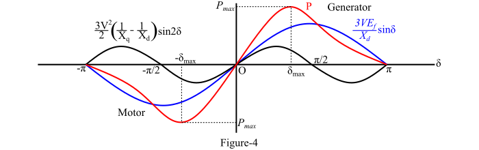
$$\mathrm{P_{3\phi} \:=\: 3P_{1\phi} \:=\:\frac{3VE_{f}}{X_{d}}\:\sin\delta \:+\:\frac{3V^{2}}{2} \left(\frac{1}{{X_{q}}} \:-\: \frac{1}{{X_{d}}}\right)\:\sin 2\delta \:\:\:\dotso\: (11)}$$
$$\mathrm{Q_{3\phi} \:=\: 3Q_{1\phi} \:=\:\frac{3VE_{f}}{X_{d}}\:\cos\delta \:-\:\frac{3V^{2}}{2X_{d}X_{q}}\left[(X_{d}\:+ \: X_{q} ) \:-\: (X_{d} \:-\: X_{q})\:\cos 2\delta \right] \:\:\:\dotso\: (12)}$$
Equations (11) & (12) are applicable to both salient-pole synchronous generator and motor. The torque angle (δ) is positive for the synchronous generator and negative for the synchronous motor.
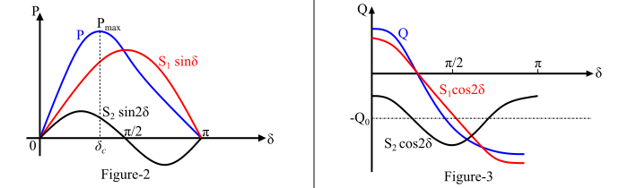
Figure-2 and Figure-3 show the (P- δ) and (Q - δ) curves respectively for a salient pole synchronous machine. Also, Figure-4 shows the power-angle curve for a salient pole synchronous machine. From the Figure-4, it is to be noted that peak-power or steady-state limit occurs at a value of δ less than 90°. The maximum value of load angle (δmax) depends upon the relative magnitudes of V, Ef and saliency.
Also, for a cylindrical rotor synchronous machine, the 3-phase real power is given by,
$$\mathrm{P_{3\phi} \:=\:\frac{3VE_{f}}{X_{d}}\:\sin\delta \:\:\:\dotso\: (13)}$$
Again, the electromagnetic torque developed by the synchronous machine is given by,
$$\mathrm{\tau_{e} \:=\:\frac{3P_{1\phi}}{\omega_{m}}\:=\: \frac{3}{2\pi n_{s}}\left[\frac{VE_{f}}{X_{d}}\:\sin\delta\:+\: \frac{V^{2}}{2} \left(\frac{1}{X_{q}} \:-\: \frac{1}{X_{d}}\right)\:\sin 2\delta \right] \:\:\:\dotso\: (14)}$$
From eqn. (13), it can be seen that the developed torque has two components – excitation torque and reluctance torque. The first term represents the torque due to field excitation and is given by,
$$\mathrm{\tau_{exc} \:=\:\frac{3VE_{f}}{2\pi n_{s}X_{d}}\:\sin\delta \:\:\:\dotso\: (15)}$$
And the second term is known as reluctance torque and is given by,
$$\mathrm{\tau_{rel} \:=\:\frac{3V^{2}}{4\pi n_{s}}\left(\frac{1}{{X_{q}}}\:-\:\frac{1}{{X_{d}}}\right)\:\sin 2\delta \:\:\:\dotso\: (16)}$$
The reluctance torque of the machine is independent of the field excitation and exists only if the synchronous machine is connected to a system receiving reactive power from other synchronous machines operating in parallel with the terminal voltage V. Actually, the reluctance torque is due to the saliency of the field poles which tend to align the direct axis with the axis of the armature MMF.