- Plotly - Home
- Plotly - Introduction
- Plotly - Environment Setup
- Plotly - Online & Offline Plotting
- Plotting Inline with Jupyter Notebook
- Plotly - Package Structure
- Plotly - Exporting to Static Images
- Plotly - Legends
- Plotly - Format Axis & Ticks
- Plotly - Subplots & Inset Plots
- Plotly - Bar Chart & Pie Chart
- Plotly - Scatter Plot, Scattergl Plot & Bubble Charts
- Plotly - Dot Plots & Table
- Plotly - Histogram
- Plotly - Box Plot Violin Plot & Contour Plot
- Plotly - Distplots, Density Plot & Error Bar Plot
- Plotly - Heatmap
- Plotly - Polar Chart & Radar Chart
- Plotly - OHLC Chart Waterfall Chart & Funnel Chart
- Plotly - 3D Scatter & Surface Plot
- Plotly - Adding Buttons/Dropdown
- Plotly - Slider Control
- Plotly - FigureWidget Class
- Plotly with Pandas and Cufflinks
- Plotly with Matplotlib and Chart Studio
- Plotly Useful Resources
- Plotly - Quick Guide
- Plotly - Cheatsheet
- Plotly - Useful Resources
- Plotly - Discussion
Scatter Plot, Scattergl Plot and Bubble Charts
This chapter emphasizes on details about Scatter Plot, Scattergl Plot and Bubble Charts. First, let us study about Scatter Plot.
Scatter Plot
Scatter plots are used to plot data points on a horizontal and a vertical axis to show how one variable affects another. Each row in the data table is represented by a marker whose position depends on its values in the columns set on the X and Y axes.
The scatter() method of graph_objs module (go.Scatter) produces a scatter trace. Here, the mode property decides the appearance of data points. Default value of mode is lines which displays a continuous line connecting data points. If set to markers, only the data points represented by small filled circles are displayed. When mode is assigned lines+markers, both circles and lines are displayed.
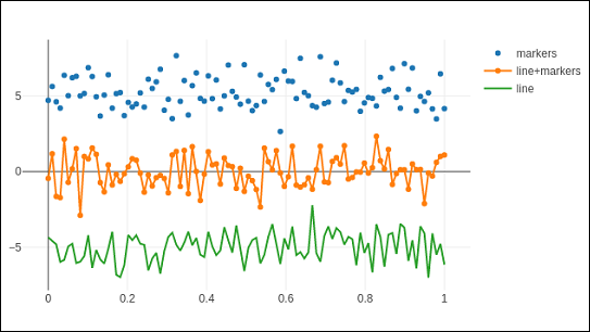
In the following example, plots scatter traces of three sets of randomly generated points in Cartesian coordinate system. Each trace displayed with different mode property is explained below.
import numpy as np
N = 100
x_vals = np.linspace(0, 1, N)
y1 = np.random.randn(N) + 5
y2 = np.random.randn(N)
y3 = np.random.randn(N) - 5
trace0 = go.Scatter(
   x = x_vals,
   y = y1,
   mode = 'markers',
   name = 'markers'
)
trace1 = go.Scatter(
   x = x_vals,
   y = y2,
   mode = 'lines+markers',
   name = 'line+markers'
)
trace2 = go.Scatter(
   x = x_vals,
   y = y3,
   mode = 'lines',
   name = 'line'
)
data = [trace0, trace1, trace2]
fig = go.Figure(data = data)
iplot(fig)
The output of Jupyter notebook cell is as given below −
Scattergl Plot
WebGL (Web Graphics Library) is a JavaScript API for rendering interactive 2D and 3D graphics within any compatible web browser without the use of plug-ins. WebGL is fully integrated with other web standards, allowing Graphics Processing Unit (GPU) accelerated usage of image processing.
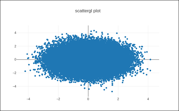
Plotly you can implement WebGL with Scattergl() in place of Scatter() for increased speed, improved interactivity, and the ability to plot even more data. The go.scattergl() function which gives better performance when a large number of data points are involved.
import numpy as np
N = 100000
x = np.random.randn(N)
y = np.random.randn(N)
   trace0 = go.Scattergl(
   x = x, y = y, mode = 'markers'
)
data = [trace0]
layout = go.Layout(title = "scattergl plot ")
fig = go.Figure(data = data, layout = layout)
iplot(fig)
The output is mentioned below −
Bubble charts
A bubble chart displays three dimensions of data. Each entity with its three dimensions of associated data is plotted as a disk (bubble) that expresses two of the dimensions through the disk's xy location and the third through its size. The sizes of the bubbles are determined by the values in the third data series.
Bubble chart is a variation of the scatter plot, in which the data points are replaced with bubbles. If your data has three dimensions as shown below, creating a Bubble chart will be a good choice.
| Company | Products | Sale | Share |
|---|---|---|---|
| A | 13 | 2354 | 23 |
| B | 6 | 5423 | 47 |
| C | 23 | 2451 | 30 |
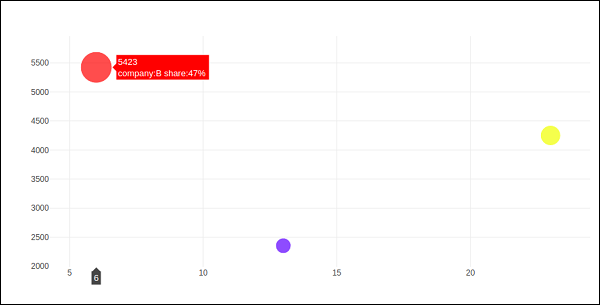
Bubble chart is produced with go.Scatter() trace. Two of the above data series are given as x and y properties. Third dimension is shown by marker with its size representing third data series. In the above mentioned case, we use products and sale as x and y properties and market share as marker size.
Enter the following code in Jupyter notebook.
company = ['A','B','C']
products = [13,6,23]
sale = [2354,5423,4251]
share = [23,47,30]
fig = go.Figure(data = [go.Scatter(
   x = products, y = sale,
   text = [
      'company:'+c+' share:'+str(s)+'%'
      for c in company for s in share if company.index(c)==share.index(s)
   ],
   mode = 'markers',
   marker_size = share, marker_color = ['blue','red','yellow'])
])
iplot(fig)
The output would be as shown below −