- Home
- Introduction
- Getting Started
- CPU and GPU
- CNTK - Sequence Classification
- CNTK - Logistic Regression Model
- CNTK - Neural Network (NN) Concepts
- CNTK - Creating First Neural Network
- CNTK - Training the Neural Network
- CNTK - In-Memory and Large Datasets
- CNTK - Measuring Performance
- Neural Network Classification
- Neural Network Binary Classification
- CNTK - Neural Network Regression
- CNTK - Classification Model
- CNTK - Regression Model
- CNTK - Out-of-Memory Datasets
- CNTK - Monitoring the Model
- CNTK - Convolutional Neural Network
- CNTK - Recurrent Neural Network
- Microsoft Cognitive Toolkit Resources
- Microsoft Cognitive Toolkit - Quick Guide
- Microsoft Cognitive Toolkit - Resources
- Microsoft Cognitive Toolkit - Discussion
CNTK - Recurrent Neural Network
Now, let us understand how to construct a Recurrent Neural Network (RNN) in CNTK.
Introduction
We learned how to classify images with a neural network, and it is one of the iconic jobs in deep learning. But, another area where neural network excels at and lot of research happening is Recurrent Neural Networks (RNN). Here, we are going to know what RNN is and how it can be used in scenarios where we need to deal with time-series data.
What is Recurrent Neural Network?
Recurrent neural networks (RNNs) may be defined as the special breed of NNs that are capable of reasoning over time. RNNs are mainly used in scenarios, where we need to deal with values that change over time, i.e. time-series data. In order to understand it in a better way, lets have a small comparison between regular neural networks and recurrent neural networks −
As we know that, in a regular neural network, we can provide only one input. This limits it to results in only one prediction. To give you an example, we can do translating text job by using regular neural networks.
On the other hand, in recurrent neural networks, we can provide a sequence of samples that result in a single prediction. In other words, using RNNs we can predict an output sequence based on an input sequence. For example, there have been quite a few successful experiments with RNN in translation tasks.
Uses of Recurrent Neural Network
RNNs can be used in several ways. Some of them are as follows −
Predicting a single output
Before getting deep dive into the steps, that how RNN can predict a single output based on a sequence, lets see how a basic RNN looks like−
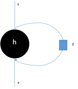
As we can in the above diagram, RNN contains a loopback connection to the input and whenever, we feed a sequence of values it will process each element in the sequence as time steps.
Moreover, because of the loopback connection, RNN can combine the generated output with input for the next element in the sequence. In this way, RNN will build a memory over the whole sequence which can be used to make a prediction.
In order to make prediction with RNN, we can perform the following steps−
First, to create an initial hidden state, we need to feed the first element of the input sequence.
After that, to produce an updated hidden state, we need to take the initial hidden state and combine it with the second element in the input sequence.
At last, to produce the final hidden state and to predict the output for the RNN, we need to take the final element in the input sequence.
In this way, with the help of this loopback connection we can teach a RNN to recognize patterns that happen over time.
Predicting a sequence
The basic model, discussed above, of RNN can be extended to other use cases as well. For example, we can use it to predict a sequence of values based on a single input. In this scenario, order to make prediction with RNN we can perform the following steps −
First, to create an initial hidden state and predict the first element in the output sequence, we need to feed an input sample into the neural network.
After that, to produce an updated hidden state and the second element in the output sequence, we need to combine the initial hidden state with the same sample.
At last, to update the hidden state one more time and predict the final element in output sequence, we feed the sample another time.
Predicting sequences
As we have seen how to predict a single value based on a sequence and how to predict a sequence based on a single value. Now lets see how we can predict sequences for sequences. In this scenario, order to make prediction with RNN we can perform the following steps −
First, to create an initial hidden state and predict the first element in the output sequence, we need to take the first element in the input sequence.
After that, to update the hidden state and predict the second element in the output sequence, we need to take the initial hidden state.
At last, to predict the final element in the output sequence, we need to take the updated hidden state and the final element in the input sequence.
Working of RNN
To understand the working of recurrent neural networks (RNNs) we need to first understand how recurrent layers in the network work. So first lets discuss how e can predict the output with a standard recurrent layer.
Predicting output with standard RNN layer
As we discussed earlier also that a basic layer in RNN is quite different from a regular layer in a neural network. In previous section, we also demonstrated in the diagram the basic architecture of RNN. In order to update the hidden state for the first-time step-in sequence we can use the following formula −
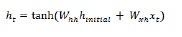
In the above equation, we calculate the new hidden state by calculating the dot product between the initial hidden state and a set of weights.
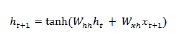
Now for the next step, the hidden state for the current time step is used as the initial hidden state for the next time step in the sequence. Thats why, to update the hidden state for the second time step, we can repeat the calculations performed in the first-time step as follows −
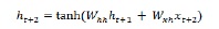
Next, we can repeat the process of updating the hidden state for the third and final step in the sequence as below −
And when we have processed all the above steps in the sequence, we can calculate the output as follows −
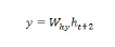
For the above formula, we have used a third set of weights and the hidden state from the final time step.
Advanced Recurrent Units
The main issue with basic recurrent layer is of vanishing gradient problem and due to this it is not very good at learning long-term correlations. In simple words basic recurrent layer does not handle long sequences very well. Thats the reason some other recurrent layer types that are much more suited for working with longer sequences are as follows −
Long-Short Term Memory (LSTM)
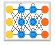
Long-short term memory (LSTMs) networks were introduced by Hochreiter & Schmidhuber. It solved the problem of getting a basic recurrent layer to remember things for a long time. The architecture of LSTM is given above in the diagram. As we can see it has input neurons, memory cells, and output neurons. In order to combat the vanishing gradient problem, Long-short term memory networks use an explicit memory cell (stores the previous values) and the following gates −
Forget gate− As name implies, it tells the memory cell to forget the previous values. The memory cell stores the values until the gate i.e. forget gate tells it to forget them.
Input gate− As name implies, it adds new stuff to the cell.
Output gate− As name implies, output gate decides when to pass along the vectors from the cell to the next hidden state.
Gated Recurrent Units (GRUs)
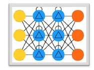
Gradient recurrent units (GRUs) is a slight variation of LSTMs network. It has one less gate and are wired slightly different than LSTMs. Its architecture is shown in the above diagram. It has input neurons, gated memory cells, and output neurons. Gated Recurrent Units network has the following two gates −
Update gate− It determines the following two things−
What amount of the information should be kept from the last state?
What amount of the information should be let in from the previous layer?
Reset gate− The functionality of reset gate is much like that of forget gate of LSTMs network. The only difference is that it is located slightly differently.
In contrast to Long-short term memory network, Gated Recurrent Unit networks are slightly faster and easier to run.
Creating RNN structure
Before we can start, making prediction about the output from any of our data source, we need to first construct RNN and constructing RNN is quite same as we had build regular neural network in previous section. Following is the code to build one−
from cntk.losses import squared_error
from cntk.io import CTFDeserializer, MinibatchSource, INFINITELY_REPEAT, StreamDefs, StreamDef
from cntk.learners import adam
from cntk.logging import ProgressPrinter
from cntk.train import TestConfig
BATCH_SIZE = 14 * 10
EPOCH_SIZE = 12434
EPOCHS = 10
Staking multiple layers
We can also stack multiple recurrent layers in CNTK. For example, we can use the following combination of layers−
from cntk import sequence, default_options, input_variable
from cntk.layers import Recurrence, LSTM, Dropout, Dense, Sequential, Fold
features = sequence.input_variable(1)
with default_options(initial_state = 0.1):
   model = Sequential([
      Fold(LSTM(15)),
      Dense(1)
   ])(features)
target = input_variable(1, dynamic_axes=model.dynamic_axes)
As we can see in the above code, we have the following two ways in which we can model RNN in CNTK −
First, if we only want the final output of a recurrent layer, we can use the Fold layer in combination with a recurrent layer, such as GRU, LSTM, or even RNNStep.
Second, as an alternative way, we can also use the Recurrence block.
Training RNN with time series data
Once we build the model, lets see how we can train RNN in CNTK −
from cntk import Function
@Function
def criterion_factory(z, t):
   loss = squared_error(z, t)
   metric = squared_error(z, t)
   return loss, metric
loss = criterion_factory(model, target)
learner = adam(model.parameters, lr=0.005, momentum=0.9)
Now to load the data into the training process, we must have to deserialize sequences from a set of CTF files. Following code have the create_datasource function, which is a useful utility function to create both the training and test datasource.
target_stream = StreamDef(field='target', shape=1, is_sparse=False)
features_stream = StreamDef(field='features', shape=1, is_sparse=False)
deserializer = CTFDeserializer(filename, StreamDefs(features=features_stream, target=target_stream))
   datasource = MinibatchSource(deserializer, randomize=True, max_sweeps=sweeps)
return datasource
train_datasource = create_datasource('Training data filename.ctf')#we need to provide the location of training file we created from our dataset.
test_datasource = create_datasource('Test filename.ctf', sweeps=1) #we need to provide the location of testing file we created from our dataset.
Now, as we have setup the data sources, model and the loss function, we can start the training process. It is quite similar as we did in previous sections with basic neural networks.
progress_writer = ProgressPrinter(0)
test_config = TestConfig(test_datasource)
input_map = {
   features: train_datasource.streams.features,
   target: train_datasource.streams.target
}
history = loss.train(
   train_datasource,
   epoch_size=EPOCH_SIZE,
   parameter_learners=[learner],
   model_inputs_to_streams=input_map,
   callbacks=[progress_writer, test_config],
   minibatch_size=BATCH_SIZE,
   max_epochs=EPOCHS
)
We will get the output similar as follows −
Output−
average  since  average  since  examples
loss      last  metric  last
------------------------------------------------------
Learning rate per minibatch: 0.005
0.4      0.4    0.4      0.4      19
0.4      0.4    0.4      0.4      59
0.452    0.495  0.452    0.495   129
[]
Validating the model
Actually redicting with a RNN is quite similar to making predictions with any other CNK model. The only difference is that, we need to provide sequences rather than single samples.
Now, as our RNN is finally done with training, we can validate the model by testing it using a few samples sequence as follows −
import pickle
with open('test_samples.pkl', 'rb') as test_file:
test_samples = pickle.load(test_file)
model(test_samples) * NORMALIZE
Output−
array([[ 8081.7905],
[16597.693 ],
[13335.17 ],
...,
[11275.804 ],
[15621.697 ],
[16875.555 ]], dtype=float32)
