- Home
- Introduction
- Getting Started
- CPU and GPU
- CNTK - Sequence Classification
- CNTK - Logistic Regression Model
- CNTK - Neural Network (NN) Concepts
- CNTK - Creating First Neural Network
- CNTK - Training the Neural Network
- CNTK - In-Memory and Large Datasets
- CNTK - Measuring Performance
- Neural Network Classification
- Neural Network Binary Classification
- CNTK - Neural Network Regression
- CNTK - Classification Model
- CNTK - Regression Model
- CNTK - Out-of-Memory Datasets
- CNTK - Monitoring the Model
- CNTK - Convolutional Neural Network
- CNTK - Recurrent Neural Network
- Microsoft Cognitive Toolkit Resources
- Microsoft Cognitive Toolkit - Quick Guide
- Microsoft Cognitive Toolkit - Resources
- Microsoft Cognitive Toolkit - Discussion
CNTK - Convolutional Neural Network
In this chapter, let us study how to construct a Convolutional Neural Network (CNN) in CNTK.
Introduction
Convolutional neural networks (CNNs) are also made up of neurons, that have learnable weights and biases. Thats why in this manner, they are like ordinary neural networks (NNs).
If we recall the working of ordinary NNs, every neuron receives one or more inputs, takes a weighted sum and it passed through an activation function to produce the final output. Here, the question arises that if CNNs and ordinary NNs have so many similarities then what makes these two networks different to each other?
What makes them different is the treatment of input data and types of layers? The structure of input data is ignored in ordinary NN and all the data is converted into 1-D array before feeding it into the network.
But, Convolutional Neural Network architecture can consider the 2D structure of the images, process them and allow it to extract the properties that are specific to images. Moreover, CNNs have the advantage of having one or more Convolutional layers and pooling layer, which are the main building blocks of CNNs.
These layers are followed by one or more fully connected layers as in standard multilayer NNs. So, we can think of CNN, as a special case of fully connected networks.
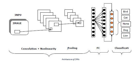
Convolutional Neural Network (CNN) architecture
The architecture of CNN is basically a list of layers that transforms the 3-dimensional, i.e. width, height and depth of image volume into a 3-dimensional output volume. One important point to note here is that, every neuron in the current layer is connected to a small patch of the output from the previous layer, which is like overlaying a N*N filter on the input image.
It uses M filters, which are basically feature extractors that extract features like edges, corner and so on. Following are the layers [INPUT-CONV-RELU-POOL-FC] that are used to construct Convolutional neural networks (CNNs)−
INPUT− As the name implies, this layer holds the raw pixel values. Raw pixel values mean the data of the image as it is. Example, INPUT [64643] is a 3-channeled RGB image of width-64, height-64 and depth-3.
CONV− This layer is one of the building blocks of CNNs as most of the computation is done in this layer. Example - if we use 6 filters on the above mentioned INPUT [64643], this may result in the volume [64646].
RELU−Also called rectified linear unit layer, that applies an activation function to the output of previous layer. In other manner, a non-linearity would be added to the network by RELU.
POOL− This layer, i.e. Pooling layer is one other building block of CNNs. The main task of this layer is down-sampling, which means it operates independently on every slice of the input and resizes it spatially.
FC− It is called Fully Connected layer or more specifically the output layer. It is used to compute output class score and the resulting output is volume of the size 1*1*L where L is the number corresponding to class score.
The diagram below represents the typical architecture of CNNs−
Creating CNN structure
We have seen the architecture and the basics of CNN, now we are going to building convolutional network using CNTK. Here, we will first see how to put together the structure of the CNN and then we will look at how to train the parameters of it.
At last well see, how we can improve the neural network by changing its structure with various different layer setups. We are going to use MNIST image dataset.
So, first lets create a CNN structure. Generally, when we build a CNN for recognizing patterns in images, we do the following−
We use a combination of convolution and pooling layers.
One or more hidden layer at the end of the network.
At last, we finish the network with a softmax layer for classification purpose.
With the help of following steps, we can build the network structure−
Step 1− First, we need to import the required layers for CNN.
from cntk.layers import Convolution2D, Sequential, Dense, MaxPooling
Step 2− Next, we need to import the activation functions for CNN.
from cntk.ops import log_softmax, relu
Step 3− After that in order to initialize the convolutional layers later, we need to import the glorot_uniform_initializer as follows−
from cntk.initializer import glorot_uniform
Step 4− Next, to create input variables import the input_variable function. And import default_option function, to make configuration of NN a bit easier.
from cntk import input_variable, default_options
Step 5− Now to store the input images, create a new input_variable. It will contain three channels namely red, green and blue. It would have the size of 28 by 28 pixels.
features = input_variable((3,28,28))
Step 6−Next, we need to create another input_variable to store the labels to predict.
labels = input_variable(10)
Step 7− Now, we need to create the default_option for the NN. And, we need to use the glorot_uniform as the initialization function.
with default_options(initialization=glorot_uniform, activation=relu):
Step 8− Next, in order to set the structure of the NN, we need to create a new Sequential layer set.
Step 9− Now we need to add a Convolutional2D layer with a filter_shape of 5 and a strides setting of 1, within the Sequential layer set. Also, enable padding, so that the image is padded to retain the original dimensions.
model = Sequential([
Convolution2D(filter_shape=(5,5), strides=(1,1), num_filters=8, pad=True),
Step 10− Now its time to add a MaxPooling layer with filter_shape of 2, and a strides setting of 2 to compress the image by half.
MaxPooling(filter_shape=(2,2), strides=(2,2)),
Step 11− Now, as we did in step 9, we need to add another Convolutional2D layer with a filter_shape of 5 and a strides setting of 1, use 16 filters. Also, enable padding, so that, the size of the image produced by the previous pooling layer should be retained.
Convolution2D(filter_shape=(5,5), strides=(1,1), num_filters=16, pad=True),
Step 12− Now, as we did in step 10, add another MaxPooling layer with a filter_shape of 3 and a strides setting of 3 to reduce the image to a third.
MaxPooling(filter_shape=(3,3), strides=(3,3)),
Step 13− At last, add a Dense layer with ten neurons for the 10 possible classes, the network can predict. In order to turn the network into a classification model, use a log_siftmax activation function.
Dense(10, activation=log_softmax)
])
Complete Example for creating CNN structure
from cntk.layers import Convolution2D, Sequential, Dense, MaxPooling
from cntk.ops import log_softmax, relu
from cntk.initializer import glorot_uniform
from cntk import input_variable, default_options
features = input_variable((3,28,28))
labels = input_variable(10)
with default_options(initialization=glorot_uniform, activation=relu):
model = Sequential([
   Convolution2D(filter_shape=(5,5), strides=(1,1), num_filters=8, pad=True),
MaxPooling(filter_shape=(2,2), strides=(2,2)),
   Convolution2D(filter_shape=(5,5), strides=(1,1), num_filters=16, pad=True),
MaxPooling(filter_shape=(3,3), strides=(3,3)),
Dense(10, activation=log_softmax)
])
z = model(features)
Training CNN with images
As we have created the structure of the network, its time to train the network. But before starting the training of our network, we need to set up minibatch sources, because training a NN that works with images requires more memory, than most computers have.
We have already created minibatch sources in previous sections. Following is the Python code to set up two minibatch sources −
As we have the create_datasource function, we can now create two separate data sources (training and testing one) to train the model.
train_datasource = create_datasource('mnist_train')
test_datasource = create_datasource('mnist_test', max_sweeps=1, train=False)
Now, as we have prepared the images, we can start training of our NN. As we did in previous sections, we can use the train method on the loss function to kick off the training. Following is the code for this −
from cntk import Function
from cntk.losses import cross_entropy_with_softmax
from cntk.metrics import classification_error
from cntk.learners import sgd
@Function
def criterion_factory(output, targets):
loss = cross_entropy_with_softmax(output, targets)
metric = classification_error(output, targets)
return loss, metric
loss = criterion_factory(z, labels)
learner = sgd(z.parameters, lr=0.2)
With the help of previous code, we have setup the loss and learner for the NN. The following code will train and validate the NN−
from cntk.logging import ProgressPrinter
from cntk.train import TestConfig
progress_writer = ProgressPrinter(0)
test_config = TestConfig(test_datasource)
input_map = {
   features: train_datasource.streams.features,
   labels: train_datasource.streams.labels
}
loss.train(train_datasource,
     max_epochs=10,
     minibatch_size=64,
     epoch_size=60000,
        parameter_learners=[learner],
     model_inputs_to_streams=input_map,
     callbacks=[progress_writer, test_config])
Complete Implementation Example
from cntk.layers import Convolution2D, Sequential, Dense, MaxPooling
from cntk.ops import log_softmax, relu
from cntk.initializer import glorot_uniform
from cntk import input_variable, default_options
features = input_variable((3,28,28))
labels = input_variable(10)
with default_options(initialization=glorot_uniform, activation=relu):
model = Sequential([
   Convolution2D(filter_shape=(5,5), strides=(1,1), num_filters=8, pad=True),
MaxPooling(filter_shape=(2,2), strides=(2,2)),
   Convolution2D(filter_shape=(5,5), strides=(1,1), num_filters=16, pad=True),
MaxPooling(filter_shape=(3,3), strides=(3,3)),
Dense(10, activation=log_softmax)
])
z = model(features)
import os
from cntk.io import MinibatchSource, StreamDef, StreamDefs, ImageDeserializer, INFINITELY_REPEAT
import cntk.io.transforms as xforms
def create_datasource(folder, train=True, max_sweeps=INFINITELY_REPEAT):
   mapping_file = os.path.join(folder, 'mapping.bin')
   image_transforms = []
   if train:
    image_transforms += [
     xforms.crop(crop_type='randomside', side_ratio=0.8),
     xforms.scale(width=28, height=28, channels=3, interpolations='linear')
]
   stream_definitions = StreamDefs(
   features=StreamDef(field='image', transforms=image_transforms),
    labels=StreamDef(field='label', shape=10)
)
   deserializer = ImageDeserializer(mapping_file, stream_definitions)
return MinibatchSource(deserializer, max_sweeps=max_sweeps)
train_datasource = create_datasource('mnist_train')
test_datasource = create_datasource('mnist_test', max_sweeps=1, train=False)
from cntk import Function
from cntk.losses import cross_entropy_with_softmax
from cntk.metrics import classification_error
from cntk.learners import sgd
@Function
def criterion_factory(output, targets):
   loss = cross_entropy_with_softmax(output, targets)
   metric = classification_error(output, targets)
return loss, metric
loss = criterion_factory(z, labels)
learner = sgd(z.parameters, lr=0.2)
from cntk.logging import ProgressPrinter
from cntk.train import TestConfig
progress_writer = ProgressPrinter(0)
test_config = TestConfig(test_datasource)
input_map = {
   features: train_datasource.streams.features,
   labels: train_datasource.streams.labels
}
loss.train(train_datasource,
     max_epochs=10,
     minibatch_size=64,
     epoch_size=60000,
        parameter_learners=[learner],
     model_inputs_to_streams=input_map,
     callbacks=[progress_writer, test_config])
Output
-------------------------------------------------------------------
average  since  average  since  examples
loss     last   metric   last
------------------------------------------------------
Learning rate per minibatch: 0.2
142      142      0.922   0.922    64
1.35e+06 1.51e+07 0.896   0.883    192
[]
Image transformations
As we have seen, its difficult to train NN used for image recognition and, they require a lot of data to train also. One more issue is that, they tend to overfit on images used during training. Let us see with an example, when we have photos of faces in an upright position, our model will have a hard time recognizing faces that are rotated in another direction.
In order to overcome such problem, we can use image augmentation and CNTK supports specific transforms, when creating minibatch sources for images. We can use several transformations as follows−
We can randomly crop images used for training with just a few lines of code.
We can use a scale and color also.
Lets see with the help of following Python code, how we can change the list of transformations by including a cropping transformation within the function used to create the minibatch source earlier.
import os
from cntk.io import MinibatchSource, StreamDef, StreamDefs, ImageDeserializer, INFINITELY_REPEAT
import cntk.io.transforms as xforms
def create_datasource(folder, train=True, max_sweeps=INFINITELY_REPEAT):
   mapping_file = os.path.join(folder, 'mapping.bin')
   image_transforms = []
   if train:
   image_transforms += [
     xforms.crop(crop_type='randomside', side_ratio=0.8),
xforms.scale(width=28, height=28, channels=3, interpolations='linear')
]
   stream_definitions = StreamDefs(
   features=StreamDef(field='image', transforms=image_transforms),
labels=StreamDef(field='label', shape=10)
)
   deserializer = ImageDeserializer(mapping_file, stream_definitions)
return MinibatchSource(deserializer, max_sweeps=max_sweeps)
With the help of above code, we can enhance the function to include a set of image transforms, so that, when we will be training we can randomly crop the image, so we get more variations of the image.
