CNTK - Classification Model

---

---

This chapter will help you to understand how to measure performance of classification model in CNTK. Let us begin with confusion matrix.

Confusion matrix

Confusion matrix - a table with the predicted output versus the expected output is the easiest way to measure the performance of a classification problem, where the output can be of two or more type of classes.

In order to understand how it works, we are going to create a confusion matrix for a binary classification model that predicts, whether a credit card transaction was normal or a fraud. It is shown as follows −

As we can see, the above sample confusion matrix contains 2 columns, one for class fraud and other for class normal. In the same way we have 2 rows, one is added for class fraud and other is added for class normal. Following is the explanation of the terms associated with confusion matrix −

• True Positives − When both actual class & predicted class of data point is 1.

• True Negatives − When both actual class & predicted class of data point is 0.

• False Positives − When actual class of data point is 0 & predicted class of data point is 1.

• False Negatives − When actual class of data point is 1 & predicted class of data point is 0.

Let’s see, how we can calculate number of different things from the confusion matrix −

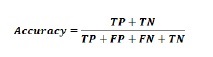
• Accuracy − It is the number of correct predictions made by our ML classification model. It can be calculated with the help of following formula −



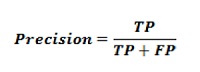
• Precision −It tells us how many samples were correctly predicted out of all samples we predicted. It can be calculated with the help of following formula −



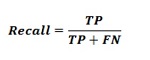
• Recall or Sensitivity − Recall are the number of positives returned by our ML classification model. In other words, it tells us how many of the fraud cases in the dataset were actually detected by the model. It can be calculated with the help of following formula −



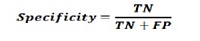
• Specificity − Opposite to recall, it gives the number of negatives returned by our ML classification model. It can be calculated with the help of following formula −

F-measure

We can use F-measure as an alternative of Confusion matrix. The main reason behind this, we can’t maximize Recall and Precision at the same time. There is a very strong relationship between these metrics and that can be understood with the help of following example −

Suppose, we want to use a DL model to classify cell samples as cancerous or normal. Here, to reach maximum precision we need to reduce the number of predictions to 1. Although, this can give us reach around 100 percent precision, but recall will become really low.

On the other hand, if we would like to reach maximum recall, we need to make as many predictions as possible. Although, this can give us reach around 100 percent recall, but precision will become really low.

In practice, we need to find a way balancing between precision and recall. The F-measure metric allows us to do so, as it expresses a harmonic average between precision and recall.

This formula is called the F1-measure, where the extra term called B is set to 1 to get an equal ratio of precision and recall. In order to emphasize recall, we can set the factor B to 2. On the other hand, to emphasize precision, we can set the factor B to 0.5.

Using CNTK to measure classification performance

In previous section we have created a classification model using Iris flower dataset. Here, we will be measuring its performance by using confusion matrix and F-measure metric.

Creating Confusion matrix

We already created the model, so we can start the validating process, which includes confusion matrix, on the same. First, we are going to create confusion matrix with the help of the confusion_matrix function from scikit-learn. For this, we need the real labels for our test samples and the predicted labels for the same test samples.

Let’s calculate the confusion matrix by using following python code −

from sklearn.metrics import confusion_matrix
y_true = np.argmax(y_test, axis=1)
y_pred = np.argmax(z(X_test), axis=1)
matrix = confusion_matrix(y_true=y_true, y_pred=y_pred)
print(matrix)

Output

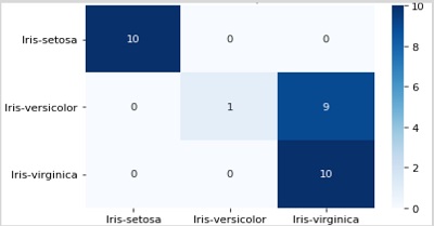
[[10 0 0]
[ 0 1 9]
[ 0 0 10]]

We can also use heatmap function to visualise a confusion matrix as follows −

import seaborn as sns
import matplotlib.pyplot as plt
g = sns.heatmap(matrix,
     annot=True,
     xticklabels=label_encoder.classes_.tolist(),
     yticklabels=label_encoder.classes_.tolist(),
     cmap='Blues')
g.set_yticklabels(g.get_yticklabels(), rotation=0)
plt.show()

We should also have a single performance number, that we can use to compare the model. For this, we need to calculate the classification error by using classification_error function, from the metrics package in CNTK as done while creating classification model.

Now to calculate the classification error, execute the test method on the loss function with a dataset. After that, CNTK will take the samples we provided as input for this function and make a prediction based on input features X_test.

loss.test([X_test, y_test])

Output

{'metric': 0.36666666666, 'samples': 30}

Implementing F-Measures

For implementing F-Measures, CNTK also includes function called fmeasures. We can use this function, while training the NN by replacing the cell cntk.metrics.classification_error, with a call to cntk.losses.fmeasure when defining the criterion factory function as follows −

import cntk
@cntk.Function
def criterion_factory(output, target):
   loss = cntk.losses.cross_entropy_with_softmax(output, target)
metric = cntk.losses.fmeasure(output, target)
   return loss, metric

After using cntk.losses.fmeasure function, we will get different output for the loss.test method call given as follows −

loss.test([X_test, y_test])

Output

{'metric': 0.83101488749, 'samples': 30}