KNIME - Building Your Own Model

In this chapter, you will build your own machine learning model to categorize the plants based on a few observed features. We will use the well-known iris dataset from UCI Machine Learning Repository for this purpose. The dataset contains three different classes of plants. We will train our model to classify an unknown plant into one of these three classes.

We will start with creating a new workflow in KNIME for creating our machine learning models.

Creating Workflow

To create a new workflow, select the following menu option in the KNIME workbench.

File → New

You will see the following screen −

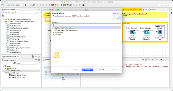
Select the New KNIME Workflow option and click on the Next button. On the next screen, you will be asked for the desired name for the workflow and the destination folder for saving it. Enter this information as desired and click Finish to create a new workspace.

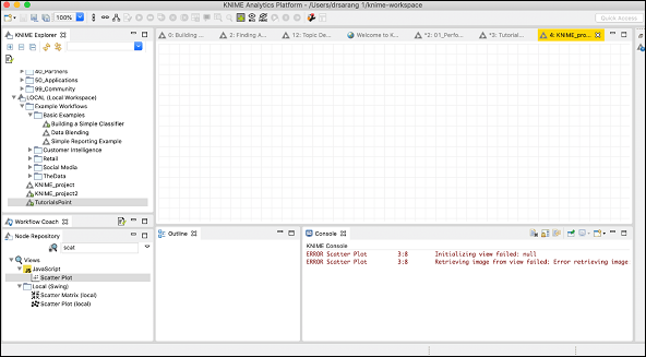
A new workspace with the given name would be added to the Workspace view as seen here −

You will now add the various nodes in this workspace to create your model. Before, you add nodes, you have to download and prepare the iris dataset for our use.

Preparing Dataset

Download the iris dataset from the UCI Machine Learning Repository site Download Iris Dataset. The downloaded iris.data file is in CSV format. We will make some changes in it to add the column names.

Open the downloaded file in your favorite text editor and add the following line at the beginning.

sepal length, petal length, sepal width, petal width, class

When our File Reader node reads this file, it will automatically take the above fields as column names.

Now, you will start adding various nodes.

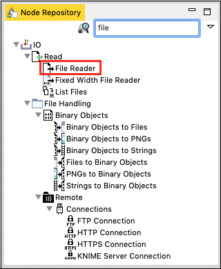
Adding File Reader

Go to the Node Repository view, type “file” in the search box to locate the File Reader node. This is seen in the screenshot below −

Select and double click the File Reader to add the node into the workspace. Alternatively, you may use drag-n-drop feature to add the node into the workspace. After the node is added, you will have to configure it. Right click on the node and select the Configure menu option. You have done this in the earlier lesson.

The settings screen looks like the following after the datafile is loaded.

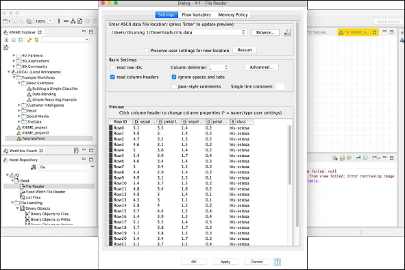
To load your dataset, click on the Browse button and select the location of your iris.data file. The node will load the contents of the file which are displayed in the lower portion of the configuration box. Once you are satisfied that the datafile is located properly and loaded, click on the OK button to close the configuration dialog.

You will now add some annotation to this node. Right click on the node and select New Workflow Annotation menu option. An annotation box would appear on the screen as shown in the screenshot here:

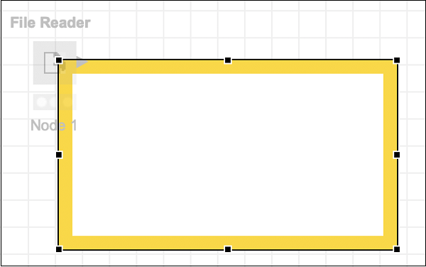
Click inside the box and add the following annotation −

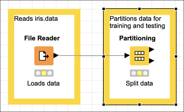
Reads iris.data

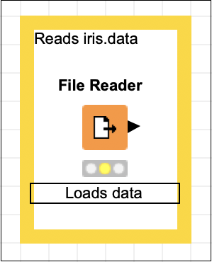
Click anywhere outside the box to exit the edit mode. Resize and place the box around the node as desired. Finally, double click on the Node 1 text underneath the node to change this string to the following −

Loads data

At this point, your screen would look like the following −

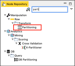
We will now add a new node for partitioning our loaded dataset into training and testing.

Adding Partitioning Node

In the Node Repository search window, type a few characters to locate the Partitioning node, as seen in the screenshot below −

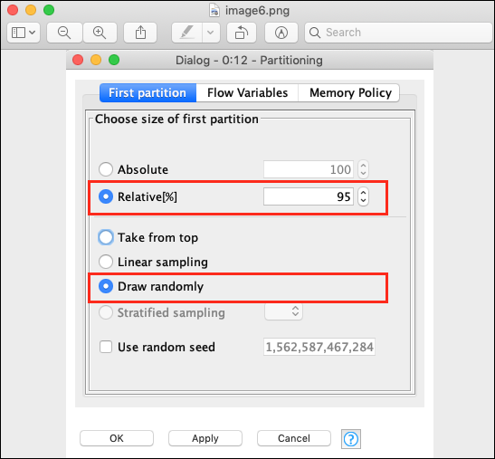
Add the node to our workspace. Set its configuration as follows −

Relative (%) : 95
Draw Randomly

The following screenshot shows the configuration parameters.

Next, make the connection between the two nodes. To do so, click on the output of the File Reader node, keep the mouse button clicked, a rubber band line would appear, drag it to the input of Partitioning node, release the mouse button. A connection is now established between the two nodes.

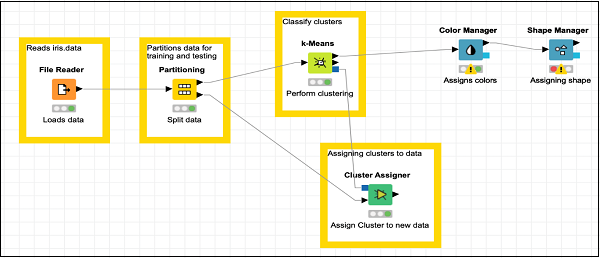
Add the annotation, change the description, position the node and annotation view as desired. Your screen should look like the following at this stage −

Next, we will add the k-Means node.

Adding k-Means Node

Select the k-Means node from the repository and add it to the workspace. If you want to refresh your knowledge on k-Means algorithm, just look up its description in the description view of the workbench. This is shown in the screenshot below −

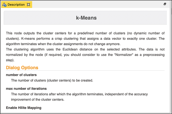
Incidentally, you may look up the description of different algorithms in the description window before taking a final decision on which one to use.

Open the configuration dialog for the node. We will use the defaults for all fields as shown here −

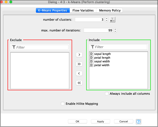
Click OK to accept the defaults and to close the dialog.

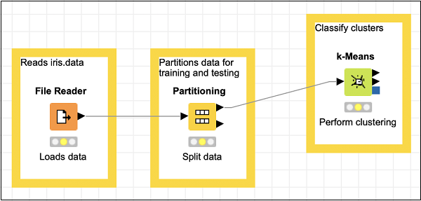
Set the annotation and description to the following −

Annotation: Classify clusters
Description:Perform clustering

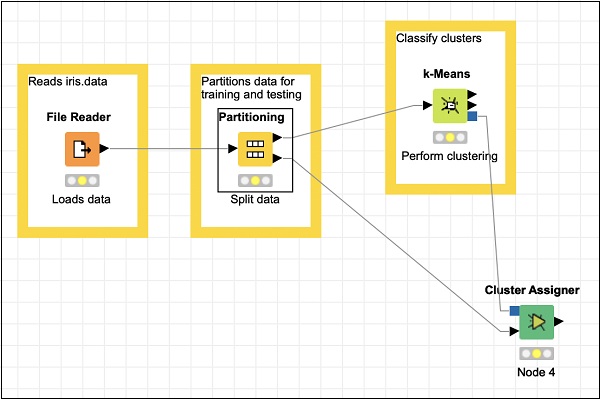
Connect the top output of the Partitioning node to the input of k-Means node. Reposition your items and your screen should look like the following −

Next, we will add a Cluster Assigner node.

Adding Cluster Assigner

The Cluster Assigner assigns new data to an existing set of prototypes. It takes two inputs - the prototype model and the datatable containing the input data. Look up the node’s description in the description window which is depicted in the screenshot below −

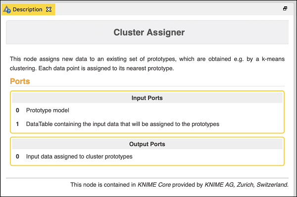
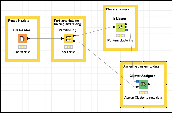
Thus, for this node you have to make two connections −

The PMML Cluster Model output of Partitioning node → Prototypes Input of Cluster Assigner
Second partition output of Partitioning node → Input data of Cluster Assigner

These two connections are shown in the screenshot below −

The Cluster Assigner does not need any special configuration. Just accept the defaults.

Now, add some annotation and description to this node. Rearrange your nodes. Your screen should look like the following −

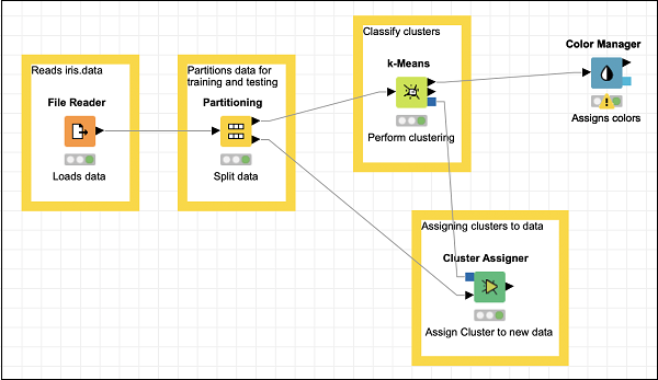
At this point, our clustering is completed. We need to visualize the output graphically. For this, we will add a scatter plot. We will set the colors and shapes for three classes differently in the scatter plot. Thus, we will filter the output of the k-Means node first through the Color Manager node and then through Shape Manager node.

Adding Color Manager

Locate the Color Manager node in the repository. Add it to the workspace. Leave the configuration to its defaults. Note that you must open the configuration dialog and hit OK to accept the defaults. Set the description text for the node.

Make a connection from the output of k-Means to the input of Color Manager. Your screen would look like the following at this stage −

Adding Shape Manager

Locate the Shape Manager in the repository and add it to the workspace. Leave its configuration to the defaults. Like the previous one, you must open the configuration dialog and hit OK to set defaults. Establish the connection from the output of Color Manager to the input of Shape Manager. Set the description for the node.

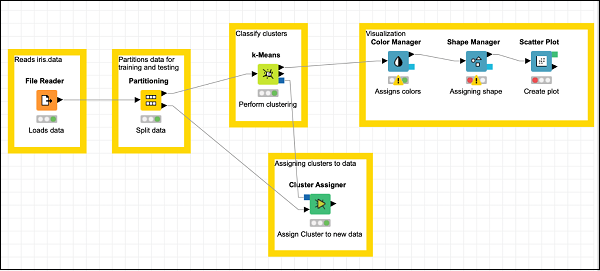
Your screen should look like the following −

Now, you will be adding the last node in our model and that is the scatter plot.

Adding Scatter Plot

Locate Scatter Plot node in the repository and add it to the workspace. Connect the output of Shape Manager to the input of Scatter Plot. Leave the configuration to defaults. Set the description.

Finally, add a group annotation to the recently added three nodes

Annotation: Visualization

Reposition the nodes as desired. Your screen should look like the following at this stage.

This completes the task of model building.