Implement Deep Autoencoder in PyTorch for Image Reconstructionp

Machine learning is one of the branches of artificial intelligence that involves developing Statistical models and algorithms that can enable a computer to learn from the input data and make decisions or predictions without being hard programmed. It involves training the ML algorithms with large datasets so that the machine can identify patterns and relationships in the data.

What is an Autoencoder?

Neural network architectures with autoencoders are used for unsupervised learning tasks. It is made up of a network of encoders and decoders that have been trained to rebuild the input data by compressing it into a lower-dimensional representation (encoding) and then decoding it to restore it to its original form.

In order to encourage the network to learn valuable characteristics or representations of the data, the objective is to minimize the reconstruction error between the input and output. Data compression, picture denoising, and anomaly detection are prominent uses for autoencoders. This reduces a lot of effort and costs associated with transferring the data.

In this article, we'll explore how to use PyTorch's Deep Autoencoder for picture reconstruction. This deep learning model will be trained on the MNIST handwritten digits, and after learning the representation of the input images, it will rebuild the digit images. A basic autoencoder consists of two main functions −

• The encoder

• The decoder

The encoder takes the input and converts the higher dimensional data to the latent low dimensional representation of the same values through a sequence of layers. This latent representation is used by the decoder to produce the reconstructed data using Python libraries torch, torch vision libraries from the PyTorch workflow, and general libraries such as numpy and matplotlib.

Algorithm

• Import all the required libraries.

• Initialize the transform operation which will be applied to every entry in the obtained dataset.

• Since tensors are necessary for Pytorch to function, we first convert each item into a tensor and normalise it to preserve the range of pixel values between 0 and 1.

• Using the torchvision.datasets program, download the dataset and save it locally in the folders./MNIST/train and./MNIST/test for the training and testing sets, respectively.

• For faster learning, convert these datasets into data loaders with batch sizes equal to 64.

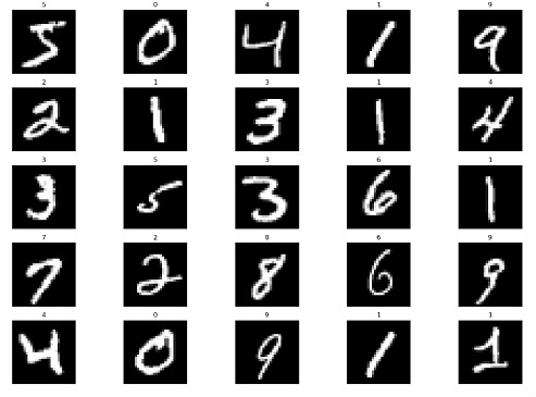
• Randomly print 25 photographs from the collection to enable us to better understand the information we are working with.

Step 1: Initialization

This step involves importing all the necessary libraries, such as numpy, matplotlib, pytorch, and torchvision.

Syntax

torchvision.transforms.ToTensor():

converts the input image (in PIL or numpy format) into a PyTorch tensor format. This transformation also scales the pixel intensities from the range [0, 255] to [0, 1].

torchvision.transforms.Normalize(mean, std)

normalizes the input image tensor with a mean and standard deviation value. This transformation helps in improving the convergence rate of the deep learning model during training. The mean and std values are usually computed from the training dataset.

torchvision.transforms.Compose(transforms)

allows chaining together multiple image transformations into a single object. This object can be passed to the PyTorch Dataset object to apply the transformations on-the-fly during training or inference.

Example

#importing modules
import numpy as np
import matplotlib.pyplot as plt
import torch
from torchvision import datasets, transforms
plt.rcParams['figure.figsize'] = 15, 10

# Initialize the transform operation
transform = torchvision.transforms.Compose([
   torchvision.transforms.ToTensor(),
   torchvision.transforms.Normalize((0.5), (0.5))
])

# Download the inbuilt MNIST data
train_dataset = torchvision.datasets.MNIST(
   root="./MNIST/train", train=True,
   transform=torchvision.transforms.ToTensor(),
   download=True)
test_dataset = torchvision.datasets.MNIST(
   root="./MNIST/test", train=False,
   transform=torchvision.transforms.ToTensor(),
   download=True)

Output

Step 2: Initializing the Autoencoder

We begin by initializing the Autoencoder class, a subclass of torch.nn.Module. We can now concentrate on creating our model architecture, which is as follows, because this abstracts away a lot of the boilerplate code for us.

Syntax

torch.nn.Linear()

A module that applies a linear transformation to the input tensor.

my_linear_layer = nn.Linear(in_features, out_features, bias=True)

torch.nn.ReLU() 

An activation function that applies the rectified linear unit (ReLU) function to the input tensor.

torch.nn.Sigmoid() 

An activation function that applies the sigmoid function to the input tensor.

Example

#Creating the autoencoder classes
class Autoencoder(torch.nn.Module):
   def __init__(self):
      super().__init__()
      self.encoder=torch.nn.Sequential(
         torch.nn.Linear(28*28,128), #N, 784 -> 128
         torch.nn.ReLU(),
         torch.nn.Linear(128,64),
         torch.nn.ReLU(),
         torch.nn.Linear(64,12),
         torch.nn.ReLU(),
         torch.nn.Linear(12,3), # --> N, 3
         torch.nn.ReLU()
      )
        
      self.decoder=torch.nn.Sequential(
         torch.nn.Linear(3,12), #N, 3 -> 12
         torch.nn.ReLU(),
         torch.nn.Linear(12,64),
         torch.nn.ReLU(),
         torch.nn.Linear(64,128),
         torch.nn.ReLU(),
         torch.nn.Linear(128,28*28), # --> N, 28*28
         torch.nn.Sigmoid()
      )
        
   def forward(self,x):
      encoded=self.encoder(x)
      decoded = self.decoder(encoded)
      return decoded

# Instantiating the model and hyperparameters
model = Autoencoder()
criterion = torch.nn.MSELoss()
num_epochs = 10
optimizer = torch.optim.Adam(model.parameters(), lr=1e-3)

Step 3: Creating a training loop

We are training an autoencoder model to learn a compressed representation of images. The training loop went through the dataset 10 times in total.

• The output of the model is computed for each batch of photos, iterating over each batch of images.

• The difference in quality between the output photos and the original pictures is then calculated.

• It averages the loss for each batch and stores the images and their outputs for each epoch.

• We depict the training loss when the loop is complete to help understand the training process.

The graphic demonstrates that the loss lowers with each passing epoch, demonstrating that the model is picking up new information and that the training procedure was successful.

The training loop trains the autoencoder model to learn a compressed representation of images by minimizing the loss between the output images and the original images. The loss decreases with each epoch, indicating successful training.

Example

# Create empty list to store the training loss
train_loss = []
# Create empty dictionary to store the images and their reconstructed outputs
outputs = {}
# Loop through each epoch
for epoch in range(num_epochs):      
   # Initialize variable for storing the running loss
   running_loss = 0      
   # Loop through each batch in the training data
   for batch in train_loader:
            
      # Load the images and their labels
      img, _ = batch
      # Flatten the images into a 1D tensor
      img = img.view(img.size(0), -1)  
      # Generate the output for the autoencoder model
      out = model(img)     
      # Calculate the loss between the input and output images
      loss = criterion(out, img)          
      # Reset the gradients
      optimizer.zero_grad()          
      # Compute the gradients
      loss.backward()          
      # Update the weights
      optimizer.step()         
      # Increment the running loss by the batch loss
      running_loss += loss.item()      
   # Calculate the average running loss over the entire dataset
   running_loss /= len(train_loader)      
   # Add the running loss to the list of training losses
   train_loss.append(running_loss)      
   # Store the input and output images for the last batch
   outputs[epoch+1] = {'input': img, 'output': out}
  
# Plot the training loss over epochs
plt.plot(range(1, num_epochs+1), train_loss)
plt.xlabel("Number of epochs")
plt.ylabel("Training Loss")
plt.show()

Output

Step 4: Visualizing

A trained autoencoder model's original and reconstructed images are plotted using this code. The variable outputs include data about the model's output, such as the reconstructed images and loss values, which were logged during various training epochs. To plot the reconstructed images from particular epochs, use the list_epochs variable.

The program plots the first five reconstructed images from the most recent batch for each of the given epochs.

Example

# Plot the re-constructed images
# Initializing the counter
count = 1
# Plotting the reconstructed images
list_epochs = [1, 5, 10]
  
# Iterate over specified epochs
for val in list_epochs:
    
   # Extract recorded information
   temp = outputs[val]['out'].detach().numpy()
   title_text = f"Epoch = {val}"
      
   # Plot first 5 images of the last batch
   for idx in range(5):
      plt.subplot(7, 5, count)
      plt.title(title_text)
      plt.imshow(temp[idx].reshape(28,28), cmap= 'gray')
      plt.axis('off')
          
      # Increment the count
      count+=1
  
# Plot of the original images
  
# Iterating over first five
# images of the last batch
for idx in range(5):
      
   # Obtaining image from the dictionary
   val = outputs[10]['img']
      
   # Plotting image
   plt.subplot(7,5,count)
   plt.imshow(val[idx].reshape(28, 28),
               cmap = 'gray')
   plt.title("Original Image")
   plt.axis('off')
      
   # Increment the count
   count+=1
  
plt.tight_layout()
plt.show()

Output

Step 5: Test Set Performance Evaluation

This code is an example of how to evaluate the performance of a trained autoencoder model on a test set.

The code concludes that the autoencoder model performed well on the test set based on the visual inspection of the reconstructed images. If the model performs well on the test set, it is likely to perform well on new, unseen data.

Example

outputs = {}
  
# Extract the last batch dataset
img, _ = list(test_loader)[-1]

img = img.reshape(-1, 28 * 28)

#Generating output
out = model(img)
  
# Storing results in the dictionary
outputs['img'] = img
outputs['out'] = out
  
# Initialize subplot count
count = 1
val = outputs['out'].detach().numpy()
  
# Plot first 10 images of the batch
for idx in range(10):
   plt.subplot(2, 10, count)
   plt.title("Reconstructed \n image")
   plt.imshow(val[idx].reshape(28, 28), cmap='gray')
   plt.axis('off')
  
   # Increment subplot count
   count += 1
# Plotting original images
# Plotting first 10 images
for idx in range(10):
   val = outputs['img']
   plt.subplot(2, 10, count)
   plt.imshow(val[idx].reshape(28, 28), cmap='gray')
   plt.title("Original Image")
   plt.axis('off')
   count += 1
  
plt.tight_layout()
plt.show()

Output

Conclusion

In conclusion, autoencoders are strong neural networks that can be applied to many different tasks, including data compression, anomaly detection, and image creation. TensorFlow, Keras, and PyTorch are a few Python tools that make autoencoder development simple. You can develop extremely potent autoencoder models by comprehending the architecture and tweaking the settings. Autoencoders are probably going to continue to be a useful tool for a variety of applications as machine learning as a field improves.