How to generate random values based on assigned probability in Excel?

In this article, the user will understand how to generate the random data value based on assigned probability in MS Excel. One example is depicted where two simple formulas are used to generate the required results. Random data would be used in multiple experiments and studies, and to analyze the available trends and patterns. For this article, the focus is to generate random values based on an assigned probability.

Example 1: To generate random value based on the assigned probability in Excel by using the user-defined formula

Step 1

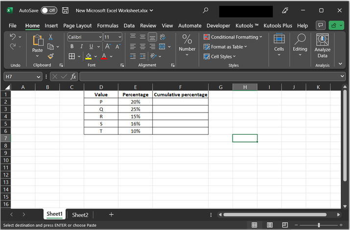
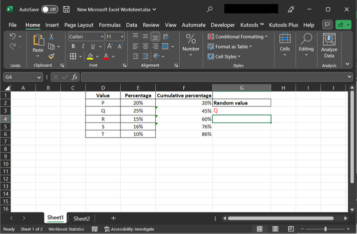
Consider the data set as shown below image:

Step 2

Go to the F2 cell, and type formula “=SUM($E$2:E2)”, as shown below.

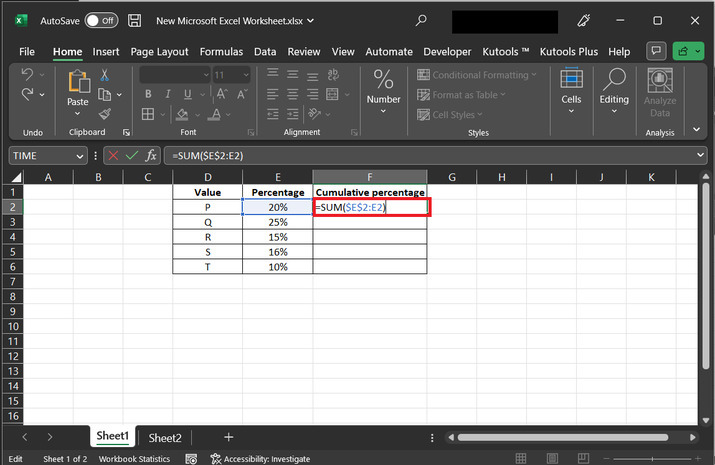
Explanation for “=SUM($E$2:E2)” formula:

• The sum is an aggregated method, to display the sum of both provided rows.

• E2, to F2, is the data range for the provided formula. As the column contains cumulative data values, cumulative values can be calculated by adding the upper column value with the side row value of the adjacent column.

After typing the above-provided formula, press the “Enter” key. This will display the result in the F2 cell.

Step 3

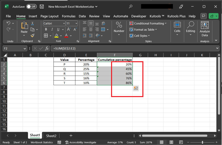
Click on the bottom corner of the F2 cell, and a plus “+” sign will appear. Drag this plus sign to the 6th row to copy the formula to all the rows. Consider the below-provided snapshot:

Step 4

Now go to the F3 cell and type the formula “ =INDEX(D$2:D$6,COUNTIF(F$2:F$6,"<="&RAND())+1)”. To generate the random value on the basis of provided data.

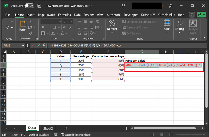
Explanation for the formula “INDEX(D$2:D$6,COUNTIF(F$2:F$6,"<="&RAND())+1)”:

• INDEX () method returns the index value for the specified data value.

• D2 to D6 is the row data that contains the data that can be generated based on random values.

• The countif () method returns the possible number of cells from the range F2:F6, that is less than or equal to the random number generated by the RAND () method.

• RAND () method generates a random number between 0 and 1.

• Adding 1 to the result ensures that the result should be generated for rows from 2 to 6.

Step 5

The above-provided formula will return “Q”, as a result. Finally, the snapshot for the code is provided below:

Please note that the example is based on random values. This simply means that every time user calls the same formula, there is a possibility that the displayed data could be different. But the displayed value should be from the range of D2 to D6, as it is the only provided range to display the required result.

Conclusion

In this article, one example is illustrated to retrieve the random value depending on the assigned probability. All the steps contain a proper detailed explanation. After following all the steps successfully user can easily evaluate the results as specified in the above steps.